7: Liquid Activity Coefficients
- Page ID
- 8145

\( \newcommand{\vecs}[1]{\overset { \scriptstyle \rightharpoonup} {\mathbf{#1}} } \)
\( \newcommand{\vecd}[1]{\overset{-\!-\!\rightharpoonup}{\vphantom{a}\smash {#1}}} \)
\( \newcommand{\dsum}{\displaystyle\sum\limits} \)
\( \newcommand{\dint}{\displaystyle\int\limits} \)
\( \newcommand{\dlim}{\displaystyle\lim\limits} \)
\( \newcommand{\id}{\mathrm{id}}\) \( \newcommand{\Span}{\mathrm{span}}\)
( \newcommand{\kernel}{\mathrm{null}\,}\) \( \newcommand{\range}{\mathrm{range}\,}\)
\( \newcommand{\RealPart}{\mathrm{Re}}\) \( \newcommand{\ImaginaryPart}{\mathrm{Im}}\)
\( \newcommand{\Argument}{\mathrm{Arg}}\) \( \newcommand{\norm}[1]{\| #1 \|}\)
\( \newcommand{\inner}[2]{\langle #1, #2 \rangle}\)
\( \newcommand{\Span}{\mathrm{span}}\)
\( \newcommand{\id}{\mathrm{id}}\)
\( \newcommand{\Span}{\mathrm{span}}\)
\( \newcommand{\kernel}{\mathrm{null}\,}\)
\( \newcommand{\range}{\mathrm{range}\,}\)
\( \newcommand{\RealPart}{\mathrm{Re}}\)
\( \newcommand{\ImaginaryPart}{\mathrm{Im}}\)
\( \newcommand{\Argument}{\mathrm{Arg}}\)
\( \newcommand{\norm}[1]{\| #1 \|}\)
\( \newcommand{\inner}[2]{\langle #1, #2 \rangle}\)
\( \newcommand{\Span}{\mathrm{span}}\) \( \newcommand{\AA}{\unicode[.8,0]{x212B}}\)
\( \newcommand{\vectorA}[1]{\vec{#1}} % arrow\)
\( \newcommand{\vectorAt}[1]{\vec{\text{#1}}} % arrow\)
\( \newcommand{\vectorB}[1]{\overset { \scriptstyle \rightharpoonup} {\mathbf{#1}} } \)
\( \newcommand{\vectorC}[1]{\textbf{#1}} \)
\( \newcommand{\vectorD}[1]{\overrightarrow{#1}} \)
\( \newcommand{\vectorDt}[1]{\overrightarrow{\text{#1}}} \)
\( \newcommand{\vectE}[1]{\overset{-\!-\!\rightharpoonup}{\vphantom{a}\smash{\mathbf {#1}}}} \)
\( \newcommand{\vecs}[1]{\overset { \scriptstyle \rightharpoonup} {\mathbf{#1}} } \)
\(\newcommand{\longvect}{\overrightarrow}\)
\( \newcommand{\vecd}[1]{\overset{-\!-\!\rightharpoonup}{\vphantom{a}\smash {#1}}} \)
\(\newcommand{\avec}{\mathbf a}\) \(\newcommand{\bvec}{\mathbf b}\) \(\newcommand{\cvec}{\mathbf c}\) \(\newcommand{\dvec}{\mathbf d}\) \(\newcommand{\dtil}{\widetilde{\mathbf d}}\) \(\newcommand{\evec}{\mathbf e}\) \(\newcommand{\fvec}{\mathbf f}\) \(\newcommand{\nvec}{\mathbf n}\) \(\newcommand{\pvec}{\mathbf p}\) \(\newcommand{\qvec}{\mathbf q}\) \(\newcommand{\svec}{\mathbf s}\) \(\newcommand{\tvec}{\mathbf t}\) \(\newcommand{\uvec}{\mathbf u}\) \(\newcommand{\vvec}{\mathbf v}\) \(\newcommand{\wvec}{\mathbf w}\) \(\newcommand{\xvec}{\mathbf x}\) \(\newcommand{\yvec}{\mathbf y}\) \(\newcommand{\zvec}{\mathbf z}\) \(\newcommand{\rvec}{\mathbf r}\) \(\newcommand{\mvec}{\mathbf m}\) \(\newcommand{\zerovec}{\mathbf 0}\) \(\newcommand{\onevec}{\mathbf 1}\) \(\newcommand{\real}{\mathbb R}\) \(\newcommand{\twovec}[2]{\left[\begin{array}{r}#1 \\ #2 \end{array}\right]}\) \(\newcommand{\ctwovec}[2]{\left[\begin{array}{c}#1 \\ #2 \end{array}\right]}\) \(\newcommand{\threevec}[3]{\left[\begin{array}{r}#1 \\ #2 \\ #3 \end{array}\right]}\) \(\newcommand{\cthreevec}[3]{\left[\begin{array}{c}#1 \\ #2 \\ #3 \end{array}\right]}\) \(\newcommand{\fourvec}[4]{\left[\begin{array}{r}#1 \\ #2 \\ #3 \\ #4 \end{array}\right]}\) \(\newcommand{\cfourvec}[4]{\left[\begin{array}{c}#1 \\ #2 \\ #3 \\ #4 \end{array}\right]}\) \(\newcommand{\fivevec}[5]{\left[\begin{array}{r}#1 \\ #2 \\ #3 \\ #4 \\ #5 \\ \end{array}\right]}\) \(\newcommand{\cfivevec}[5]{\left[\begin{array}{c}#1 \\ #2 \\ #3 \\ #4 \\ #5 \\ \end{array}\right]}\) \(\newcommand{\mattwo}[4]{\left[\begin{array}{rr}#1 \amp #2 \\ #3 \amp #4 \\ \end{array}\right]}\) \(\newcommand{\laspan}[1]{\text{Span}\{#1\}}\) \(\newcommand{\bcal}{\cal B}\) \(\newcommand{\ccal}{\cal C}\) \(\newcommand{\scal}{\cal S}\) \(\newcommand{\wcal}{\cal W}\) \(\newcommand{\ecal}{\cal E}\) \(\newcommand{\coords}[2]{\left\{#1\right\}_{#2}}\) \(\newcommand{\gray}[1]{\color{gray}{#1}}\) \(\newcommand{\lgray}[1]{\color{lightgray}{#1}}\) \(\newcommand{\rank}{\operatorname{rank}}\) \(\newcommand{\row}{\text{Row}}\) \(\newcommand{\col}{\text{Col}}\) \(\renewcommand{\row}{\text{Row}}\) \(\newcommand{\nul}{\text{Nul}}\) \(\newcommand{\var}{\text{Var}}\) \(\newcommand{\corr}{\text{corr}}\) \(\newcommand{\len}[1]{\left|#1\right|}\) \(\newcommand{\bbar}{\overline{\bvec}}\) \(\newcommand{\bhat}{\widehat{\bvec}}\) \(\newcommand{\bperp}{\bvec^\perp}\) \(\newcommand{\xhat}{\widehat{\xvec}}\) \(\newcommand{\vhat}{\widehat{\vvec}}\) \(\newcommand{\uhat}{\widehat{\uvec}}\) \(\newcommand{\what}{\widehat{\wvec}}\) \(\newcommand{\Sighat}{\widehat{\Sigma}}\) \(\newcommand{\lt}{<}\) \(\newcommand{\gt}{>}\) \(\newcommand{\amp}{&}\) \(\definecolor{fillinmathshade}{gray}{0.9}\)Distillation Science (a blend of Chemistry and Chemical Engineering)
This is Part VII, Liquid Activity Coefficients of a ten-part series of technical articles on Distillation Science, as is currently practiced on an industrial level. See also Part I, Overview for introductory comments, the scope of the article series, and nomenclature.
Part VII, Liquid Activity Coefficients builds on Part VI, Fugacity regarding the departure of vapor-liquid equilibria (VLE) of binary mixtures from ideal behavior, as is commonly found in practical application of distillation science. In conjunction with previous articles, the goal of this article to to complete the explanation of equilibrium behavior of binary systems; such that Part IX can illustrate an example of a distillation process design.
In Part VI the combination of Raoult’s Law and Dalton’s Law was introduced governing the ideal vapor-liquid behavior of volatile fluid mixtures, with Equation 6-1 repeated for convenience.
\( Y_{1}=(X_{1} \times VP_{1})/(X_{1} \times VP_{1} + X_{2} \times VP_{2}) \nonumber\) \( Y_{2}=(X_{2} \times VP_{2})/(X_{1} \times VP_{1} + X_{2} \times VP_{2}) \nonumber\) repeat Equation 6-1
Also in Part VI the real-world departure from ideal behavior was discussed as far as the fugacity coefficients, but stopped short of Liquid Activity Coefficients. Equation 6-4 repeated below gave the complete relationship between the partial pressure of the ith component, PPi, and the pure-component vapor pressure VPi , for liquid and vapor mole fractions Xi and Yi, respectively. The total system pressure (sum of the partial pressures) is denoted as \(\pi \nonumber\); (\(\phi_{i}^V\nonumber\)& \(\phi_{i}^L\nonumber\)) are the liquid and vapor fugacity coefficients. \(\gamma_{i} \nonumber\) is the ith component’s Liquid Activity Coefficient for that specific set of components.
\(Y_{i} \times \pi =PP_{i} =(\phi_{i}^L/ \phi_{i}^V) \times \gamma_{i} \times VP_{i} \times X_{i} \nonumber\) repeat Equation 6-4
An example was given in Part VI of a vaporizing TCS-STC mixture, contrasting the vapor-liquid equilibria (VLE) expected from Raoult/Dalton; from what actually occurs in the real world as a result of the ideality departures. Summarizing the previous article, the more volatile fluid exerts an effect on the less volatile fluid, to increase its apparent vapor pressure; and the less volatile fluid reduces the more volatile fluid’s vapor pressure. The net effect is to make the component separations more difficult via distillation (e.g., more theoretical trays or increased amount of reflux than expected). For detailed discussion of fugacity coefficients, see Part VI.
As a “house-keeping” note, it must be emphasized that Parts VI and VII treat fugacity coefficients and Liquid Activity Coefficients separately. In some texts, the two topics are compressed together using specific models of mixing and Equations of State (EOS). However, the two ideality departure factors are differently based, and their combination often gives erroneous or nonsense results when used with polar fluids, or those that have a high degree of hydrogen bonding (such as the chlorosilanes that are used as continuing examples). Fugacity coefficients naturally result from differences in fluid volatility. Liquid Activity Coefficients result from differences in fluid properties, including critical temperature (Tc), critical pressure (Pc), critical volume (Vc) and acentric factor (ω), as well as the entropy & enthalpy effects of mixing (referred to in thermodynamic texts as excess Gibbs Free Energy).
For a given temperature and combination of fluids, the value of \(\gamma \nonumber\) is a function of the liquid mole fraction, rising asymptotically from unity at the pure component condition. Typically the values of \(\gamma \nonumber\) for a system are plotted as a function of the more volatile component’s mole fraction. An example of such a plot is given in Figure 7-1, for the TCS-STC binary at 73.9°C (the temperature of the continuing example of previous articles).
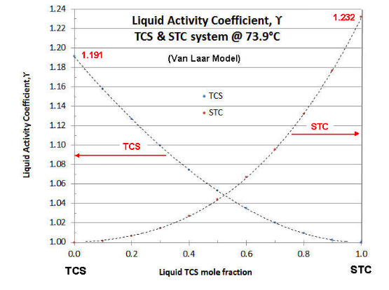
There are several models for Liquid Activity Coefficients that are thermodynamically consistent (i.e., follow the Gibbs-Duhem Rule of binary system thermodynamics). The two-constant Van Laar model is the easiest to manipulate, but is limited to binary systems. The Margules model is not that different from the Van Laar model, and also limited to binary systems. The Wilson model is more complex mathematically, but can be applied to ternary or greater-numbered component systems. Fortunately the Wilson model parameters can be calculated from the Van Laar model. Even more complex Liquid Activity Coefficient models are known (e.g., NRTL and UNIQUAC), but these require more data points to effectively evaluate. In the case of the above plot, the Van Laar model is shown. In Part VIII, the techniques are discussed to evaluate experimental data on Liquid Activity Coefficients and fit the data to a model. In most cases with chlorosilanes (and their impurities) the data quality is not that great, so the simpler Van Laar is typically used to correlate data and for evaluating binary systems, and the Wilson model is used for ternary systems and beyond. For a more in-depth discussion of Liquid Activity Coefficients, the reader is referred to the text " The Properties of Gases and Liquids", by Reid, Prausnitz and Sherwood, (McGraw-Hill). The third edition is more readable, but the fifth edition is more updated.
The Van Laar model is:
\[Ln(\gamma_{1}) =A_{1} \times [1+(A_{1} \times X_{1})/(A_{2} \times X_{2})]^{-2} \label{7-1} \]
\(Ln(\gamma_{2}) =A_{2} \times [1+(A_{2} \times X_{2})/(A_{1} \times X_{1})]^{-2} \nonumber\)
with A1 and A2 being the Van Laar constants for the more volatile and less volatile component, respectively.
Conveniently, \[EXP(A_{1}) = \gamma_{1} @ X_{2} \rightarrow 0 \label{7-2} \]
\(EXP(A_{2}) = \gamma_{2} @ X_{1} \rightarrow 0 \nonumber\)
which simplifies evaluation. Note from Figure 7-1 that the Liquid Activity Coefficients plot is not always symmetrical (i.e., A1≠ A2). In the plot of Figure 7-1, A1 (TCS) = 0.1752, so the TCS curve asymptotes at \(\gamma \nonumber\)= 1.191; and A2 (STC) = 0.2086, so the TCS curve asymptotes at \(\gamma \nonumber\)= 1.232 .
Completing the on-going example from Part VI, for a TCS-STC liquid mixture, with 40% molar TCS, at 73.9°C, to determine the vapor mole fraction in equilibrium (but now including the Liquid Activity Coefficient effects):
In Part VI, the pure-component vapor pressures of TCS and STC respectively were calculated from the VP equation of Part IV to be 3.500 and 1.651 atmospheres, respectively at 73.9°C. Also from Part V, the liquid and vapor fugacities were calculated as per Table 6-1, repeated below, using the Peng-Robinson EOS (Part V).
|
TCS |
STC |
|
|---|---|---|
|
\(\phi^L \nonumber\) |
0.9976 |
1.0039 |
|
\(\phi^V \nonumber\) |
1.0488 |
0.9562 |
|
\(\phi^L / \phi^V \nonumber\) |
0.9512 |
1.0498 |
The values for \(\gamma \nonumber\) are calculated for TCS and STC @ 0.40 mf TCS, per Equation (\ref{7-1}) using the values for A1 and A2 above (or just read from Figure 7-1), to be 1.075 and 1.027 respectively. Plugging all these values into Equation 6-4 (repeated above), the partial pressures of TCS and STC @ 73.9°C are:
\(PP_{TCS} =0.9512 \times 1.075 \times 3.500 \times 0.40 =1.432 \nonumber\) atmospheres, and
\(PP_{STC} =1.0498 \times 1.027 \times 1.651 \times 0.60 =1.068 \nonumber\) atmospheres.
So the value of \(Y_{TCS} = 1.432/(1.432+1.068) =.573 \nonumber\), which was given in Part VI, with the STC mole fraction being 0.427.
The careful reader will see that not only are the partial pressures of TCS and STC different from Raoult/Dalton, but so is the total pressure. In the ideal behavior of Raoult/Dalton, the partial pressures were given in Part VI as 1.400 and 0.991 atmospheres, for a total pressure of 2.39 atmospheres. But in reality, at 73.9°C and 0.40 mf TCS, the total pressure would instead be 2.50 atmospheres. So while the ideality departures of TCS made the vapor mole fraction smaller (0.573 vs 0.586), both the TCS and STC exerted slightly more partial pressure than Raoult would indicate. But the TCS mole fraction still went down, because the ideality departure of STC was greater than that of TCS.
The take-away from this example is that while Raoult/Dalton will give you a “quick & dirty” value for Y/X, it is easy to get the overall wrong answer for determining the requirements of a distillation column design. In almost every instance of industrial practice, the use of Raoult/Dalton will undersize the number of trays needed to make a separation (or for the same number of trays, undersize the reflux required). For this reason, it is important to know how to work out the better answer.
For many binary systems, VLE data exists – but typically not at the temperature/pressure needed for industrial design. Most industrial designs use higher pressures for economy of size, as well as to accommodate available energy sources for driving the column reboiler and condenser. Yet the practicalities of data collection in the laboratory usually require pressures slightly above ambient, or at slight vacuums. This is especially true of chlorosilanes, since the normal materials of construction for higher pressures can catalyze slow side reactions, such as disproportionation and dimerization.
Lab data is normally collected based on small amounts of fluid that are used repeatedly at somewhat different combinations of temperature and composition. In the case of electronic impurities, some of these compounds are not very stable outside of a chlorosilane matrix. So a correlating method must be used that allows a certain degree of extrapolation.
In 1981 Chung-Ton Lin and Thomas Daubert from Penn State University developed such a Liquid Activity Coefficient model and published same in Industrial & Engineering Chemistry Process Design and Development, basing their work on non-polar hydrocarbon mixtures. I have used their general method, but modified two of the constants so as to better fit available VLE data on chlorosilanes. Using these re-evaluated constants, the revised “Lin & Daubert” method (detailed below as Equation (\ref{7-3}) was used to check against industrially obtained data on the distillation purification of TCS and silane, with good results. Obviously more data would be preferable, especially on ternary mixtures and low-concentration electronic impurities in chlorosilanes. However until such becomes available, Equation (\ref{7-3}) below is recommended.
To develop a generic expression for the Van Laar parameters (\(A_{i} \nonumber\) & \(A_{j} \nonumber\) ), Lin & Daubert go back to Van Laar’s original two-term expression regarding the excess Gibbs energy of mixing, using the SRK Equation of State for partial molar compressibility and simple mixing rules; and expand it into the following:
\[A_{i} = c \times F_{i} +d \times k_{ij} \times G_{i} \label{7-3} \]
\(A_{j} = c \times F_{j} +d \times k_{ij} \times G_{j} \nonumber\)
- \(F_{i} =1/[T_{ri}P_{ci}] \times (R_{i} \times (1+M_{j})^{0.5} \times P_{ci}^{0.5} - R_{j} \times (1+M_{j})^{0.5} \times P_{cj}^{0.5})^2 \nonumber\)
- \(F_{j} =1/[T_{rj}P_{cj}] \times (R_{j} \times (1+M_{i})^{0.5} \times P_{cj}^{0.5} - R_{i} \times (1+M_{i})^{0.5} \times P_{ci}^{0.5})^2 \nonumber\)
- \(G_{i} = T_{ri}^{-1} (P_{cj}/P_{ci})^{0.5} \times R_{i} \times (1+M_{i})^{0.5} \times R_{j} (1+M_{i})^{0.5} \nonumber\)
- \(G_{j} = T_{rj}^{-1} (P_{ci}/P_{cj})^{0.5} \times R_{j} \times (1+M_{j})^{0.5} \times R_{i} (1+M_{j})^{0.5} \nonumber\)
- \(M_{i} = 0.480 + 1.574\omega_{i} -.176\omega_{i}^2 \nonumber\) \(M_{j} = 0.480 + 1.574\omega_{j} -.176\omega_{j}^2 \nonumber\)
- \(R_{i} =[1+M_{i} \times (1-T_{ri}^{0/5})]^{0.5} \nonumber\) \(R_{j} =[1+M_{j} \times (1-T_{rj}^{0/5})]^{0.5} \nonumber\)
- \(k_{ij} =1 - 2 \times [V_{ci}^{1/3} \times V_{cj}^{1/3}]^{0.5} / [V_{ci}^{1/3} + V_{cj}^{1/3}] \nonumber \)
Using an improved set of curve-fits for “c”,
- \(0< \Delta \omega <0.03 ⇒ \nonumber\)\( Ln(c)= -8.0637E+04(\Delta \omega)^3 +8.2649E+03(\Delta \omega)^ 2 - 3.2891E+02 (\Delta \omega) +5.5051 \nonumber\)
- \(0.03 < \Delta \omega <0.30 ⇒ \nonumber\)\( Ln(c)=6.4645E+02(\Delta \omega)^4 -7.9857E+02(\Delta \omega)^3 +3.4768E+02(\Delta \omega)^2 -6.5099E+01(\Delta \omega) +2.5667 \nonumber\)
Reducing available VLE data to Van Laar parameters, and adjusting for vapor and liquid fugacity coefficients, the best value of “d” is found to be 112.1 for chlorosilanes and similar fluids.
Lin & Daubert suggested that the “c” function be capped at \(0.005 < \Delta \omega=|\omega_{i} - \omega_{j}| <0.15 \nonumber\), based on their data; but using the above improved set of polynomials for “c” avoids singularities during iterative calculations, with a minimum “c” of 0.135 (as “Δω” → ∞ )
Note that the "c" variable in the first term of Equation 7-3 is based on the \(F_{i} \nonumber\) values and the differences between the two fluid's acentric factor, ω ( i.e., their molecular complexity); whereas the second term of Equation 7-3 is based on the \(G_{i} \nonumber\) values and the differences between the two fluid's molecular volumes at critical (Vc).
Returning to the continuing previous TCS-STC example, and using the two components’ critical temperature (Tc), critical pressure (Pc), critical volume (Vc) and acentric factor (ω), as well as basing the reduced temperature (Tr) on 73.9°C = 347.05°K, Equation (\ref{7-3}) gives the values of A1 and A2 used earlier in this article, of 0.1752 and 0.2086 respectively.
Frequently in evaluating different distillation designs for a process, the designer is faced with the need to make process temperature changes and determine the effect on Y/X using Equation 6-4, repeated above. That causes no problem in the evaluation of the fugacity ratio,\(\phi_{i}^L / \phi_{i}^V \nonumber\), since those factors are derived from the EOS ( see Part VI). However, if using experimentally obtained values for \(\gamma \nonumber\) that were obtained at a different temperature, there needs to be further adjustment. The general “rule-of-thumb” seen in some texts is that Ln(\(\gamma \nonumber\)) is proportional to 1/T (absolute temperature) for small temperature changes. In reality such a “rule-of-thumb” is tantamount to making an assumption that the mixing effects of the multi-component fluid are closer to an isothermal model than an isenthalpic one. In most cases, the temperature dependency on activity coefficient is a blend of two theoretical models, which leads to the relationship:
\[Ln(\gamma_{i})=a + \frac{b}{T} \label{7-4} \]
where “a” and “b” are the constants of a linear relationship (“a” = 0 leading to the isenthalpic model, or “b” = 0 leading to the isothermal model). The use of Equation (\ref{7-3}) solves the problem, since it predicts such temperature changes along the lines of Equation (\ref{7-4}) , and so can be used in a relative manner. For example, if Equation (\ref{7-3}) is found to over-predict the value of \(Ln(\gamma) \nonumber\) by 10% of an experimentally obtained activity coefficient value, then calculate how much Equation (\ref{7-3}) would predict for the different temperature, and apply that 10% on the \(Ln(\gamma) \nonumber\).
Note that to all intents, the Liquid Activity Coefficient is not a direct function of pressure, other than increasing the boiling temperature increases pressure. However, fugacities are a function of both temperature and pressure, and that is why they should be included in Y/X calculations (many texts advocate setting fugacities to unity, which is only close to being valid at very low pressures).
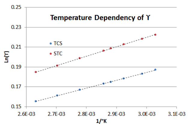
To demonstrate how Equation (\ref{7-3}) performs with changing temperature (from 330°K to 380°K), Figure 7-2 shows the dependency for the asymptotic BIP’s of the TCS-STC mixture in the example above. Note that the slope of the STC Liquid Activity Coefficient line is about 20% steeper than that of the TCS Liquid Activity Coefficient line (i.e., in the TCS-STC binary system, increasing the temperature has a greater effect on the STC's \(\gamma \nonumber\) than it does on the TCS's \(\gamma \nonumber\)).