9: Putting It All Together

Distillation Science (a blend of Chemistry and Chemical Engineering)

This is Part IX, Putting It All Together of a ten-part series of technical articles on Distillation Science, as is currently practiced on an industrial level. See also Part I, Overview for introductory comments, the scope of the article series, and nomenclature.

Part IX, Putting It All Together uses the information from Parts III through VII, showing how to combine them in a practical example for bulk separation; and how using the techniques detailed in previous articles give answers that differ from the ideals of basic Raoult/Dalton Law application.

See previous articles per the following detail:

• Part III for critical properties and acentric factor, especially Table 3-3
• Part IV for the recommended vapor pressure equation, especially Equation 4-3 and Table 4-1
• Part V for Equation of State, especially Equations 5-3 and 5-4
• Part VI, especially Equation 6-4 for partial pressure and Equations 6-7 and 6-8 for fugacity coefficients
• Part VII for Liquid Activity Coefficients, especially Equation 7-3

In this article a practical distillation example is developed, showing the Y/X relationship with temperature for the DCS-TCS binary system with pressure is held constant at 11.0 atmospheres, and showing the results as a TXY/P plot as well as in tabular form. From such data, a distillation column designer would consider the best arrangement for column feed, “tops” and “bottoms” recovery, tray count and external reflux ratio ( and from that, the energy required for the reboiler and condenser, as well as hydraulic loading per unit mass flow of feedstock). Two variations of this example are worked-up, showing the application of distillation science: one which only uses ideal Raoult/Dalton, and one that uses the full set of ideality departure coefficients. Table output and plots below are done using MS Excel. Then at the end of the article, the table results are graphically demonstrated using a McCabe-Theile plot to step off the trays for an appropriate reflux rate and show the best feed tray.

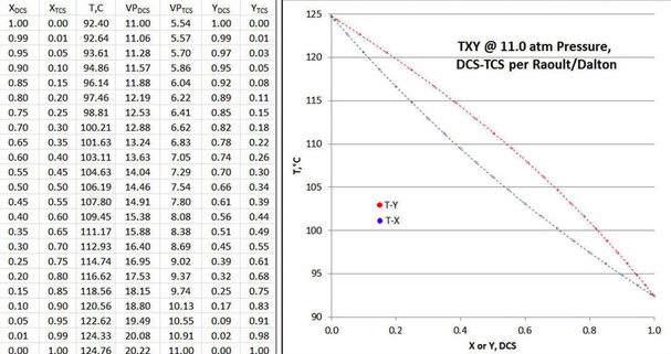
The table of Figure 9-1 is set up to cover the range of DCS liquid mole fraction from unity to zero, in increments of 0.05 mole fraction, with 0.01/0.99 mole fraction added to illustrate asymptotic effects. For each non-zero table row, a temperature is first assumed, and then the vapor mole fractions calculated per Raoult/Dalton, with p=11.0 atmospheres; then that row’s temperature is iteratively adjusted until the total pressure = 11.0 atmospheres.

In the plot of Figure 9-1 shows the calculation results in TXY/P form, with the value of X_DCS=1.0 representing the tightest possible “tops” product at the distillation column condenser; and a value of X_DCS=0.0 representing the tightest possible “bottoms” product at column reboiler, all at a total reflux condition. For a finite column, the mole fraction of the “tops” product would be a cropping of the upper X_DCS values of the TXY/P curves; and the mole fraction of the “bottoms” product a would be a cropping of the lesser X_DCS values of the TXY/P curves. In such instance, the column feed tray would be identified as that point in the column where the tray temperature is identical to the feed mixture’s boiling point. The accompanying plot of solution shows what the TXY/P curves would look like, for such a Raoult/Dalton solution to the DCS-TCS binary at 11.0 atmospheres.

\( Y_{1}=(X_{1} \times VP_{1})/(X_{1} \times VP_{1} + X_{2} \times VP_{2}) \nonumber\) \( Y_{2}=(X_{2} \times VP_{2})/(X_{1} \times VP_{1} + X_{2} \times VP_{2}) \nonumber\) repeat Equation 6-1

Figure 9-1, TXY calculation table and plot, Raoult/Dalton

If the data plot of Figure 9-1 plot is carefully examined, one can see that the T-X and T-Y curves are exactly symmetrical when “folded” along a line running from abscissa/ordinate points of (0,124.76) to (1,92.40); or “folded” orthogonally to that same line. In other words, there are no departures from ideality in either vapor or liquid phase, either with DCS or TCS.

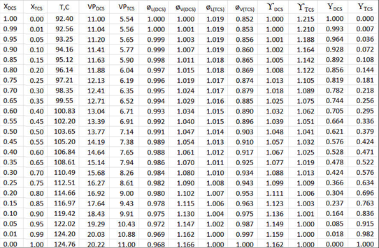
Now X and Y are re-calculated including the departures from ideality, both in fugacity (ø) as well as Liquid Activity Coefficients ( \(\gamma \nonumber\) ).

Figure 9-2, TXY/P calculation table, all departure factors included

The table in above Figure 9-2 is likewise set up and calculations performed row-wise for each value of X_DCS, but the liquid and vapor-phase fugacity coefficients (ø_L and ø_V) and activity coefficients ( \(\gamma_{i} \nonumber\) ) are included in the calculation of vapor mole fractions (\(\gamma_{DCS} \nonumber\) ). For each row, the temperature is iterated until the sum of partial pressures = 11.0 atmospheres. Note that since the activity coefficients are mild functions of temperature, each row has its own Van Laar constants determined and the value of \(\gamma \nonumber\) calculated for that row’s liquid mole fraction. Thus all departure-from-ideality factors are included.

\[ Y_{i}= (\phi_{i}^L \times \gamma_{i} \times VP_{i} \times X_{i})/(\phi_{i}^V \times \pi) \label{9-1} \]

which is an algebraic re-arrangement of Equation 6-4 from previous Part VI.

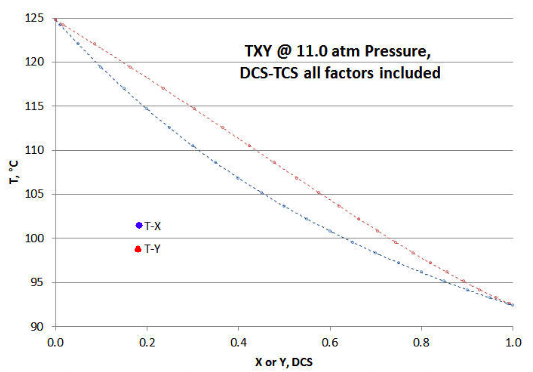
To better show how the several ideality departure factors impact the TXY/P plot (as compared to Figure 9‑1 above), the table in Figure 9-2 is plotted. The symmetry of the Figure 9-1 Raoult/Dalton plot is no longer there, neither along the “fold” line running from abscissa/ordinate points of (0,124.76) to (1, 92.40); or “folded” orthogonally to that same line. Also note that the T-X and T-Y curves are closer together in Figure 9‑3, as opposed to Figure 9-1.

Figure 9-3, TXY/P plot, all departure factors included

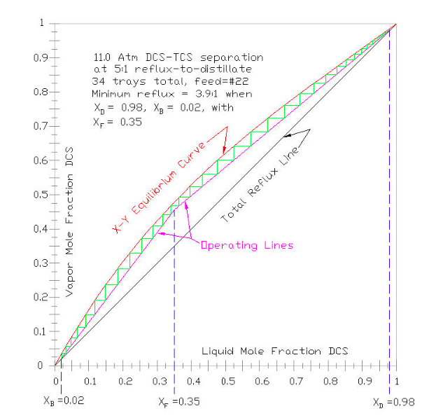
For a very simple approximation of tray count, for given distillation column “tops” product , “bottoms” product and feed mixture mole fractions, and for a given reflux rate, a McCabe-Thiele plot is constructed in Figure 9-4 to graphically step off the number of trays above and below the feed tray. For almost all industrial applications, this tray-by-tray analysis is done via computer modeling, such as ASPEN, VMG, HYSYS, ChemCad, etc. To apply the technique to a computer model, the user would specify the critical constants ( as per Part III), the vapor pressure equation to be used (as per Part IV), the EOS to be used to calculate fugacity coefficients (as per Part V), and the Liquid Activity Coefficient model to be used (as per Part VI).

To construct a McCabe-Thiele plot, the X-Y equilibrium (in red below) is plotted on a set of axes where X= liquid mole fraction of the most volatile component = X_DCS ; and Y= vapor mole fraction of the most volatile component = Y_DCS . The total reflux line (in black below) connects (X,Y) = (0,0) and (1,1); representing the maximum reflux possible. The lines are added (in dashed blue below) for the feed (X_F), and distillate product (X_D) and the bottoms product (X_B), from the X-axis to the total reflux line. The feed line is extended toward the equilibrium curve, and from that intersection a line is drawn to the end of the distillate product line. The slope of that drawn line represents the minimum internal reflux needed to make the separation (i.e., with an infinite number of trays). The upper column operating line (in magenta below) is then drawn connecting the end of the distillate product line with the feed line, with a slope somewhat greater than the minimum reflux slope. In normal practice the upper column operating line slope is usually about 1.3 times the minimum slope, depending on the relative value of operating energy vs capital cost. Then the lower column operating line is drawn, intersecting the bottoms product line with the upper column operating line (and the feed line). The number of theoretical trays (aka stages) can then be stepped off ( in green below) from X_D to X_B, and best tray determined for the feed.

Figure 9-4, McCabe Thiele solution to example calculations

To illustrate an example of using a McCabe-Thiele plot, assume the mixture to be separated is a 35% DCS molar liquid, pre-heated to its boiling point of 108.61°C (as shown on the 35% of Figure 9-2). Further, assume that the column “tops” distillate product is to be 98% molar DCS and the column “bottoms” product is to be 98% molar TCS. Per the text above, the minimum reflux (i.e., the slope of the line between X_D = X_DCS of 0.98, X_B = X_DCS of 0.02) is determined to be 3.9:1, reflux-to-distillate. To allow a reasonable number of trays, a reflux rate of 5:1 is chosen (about 1.3 times the minimum), so the slope of the upper column operating line is R/(R+1) = 5/(5+1) =0.8333. Stepping off trays, it is determined that the total number of theoretical trays required is 34, with the feed tray at #22. Conventional tray counting starts at the column condenser = tray #1.

As can be seen by examining Figure 9-4, as the column’s reflux rate is increased, upper column (magenta) operating line’s slope increases, and the gap opens up between the (red) X-Y Equilibrium Line and the (black) Total Reflux Line. So increasing the reflux decreases the number trays required to make the specified separation.

In a normal industrial process application, all of the calculations are done via computer simulators, allowing for variations in operating line slope; feed quality condition (e.g., saturated vapor, saturated liquid, sub-cooled liquid, etc); changes in the internal liquid/vapor flow ratios due to physical properties; ambient heat effects; tray efficiencies, etc; as well as integrating the distillation column into the rest of the process design. So the McCabe-Thiele method is just used for graphical explanation.

However, the primary consideration of the distillation column design is the X-Y equilibrium relationship. If this is considerably in error – such as using only Raoult/Dalton – the column design will be a failure. Given the cost of industrial-scale distillation systems being in the millions of dollars (tens of $MM for larger ones), there is every reason to get the X-Y equilibrium relationship correct.

In the example of this article, the basic Raoult/Dalton model would result in the X-Y equilibrium relationship in the above example having more curvature (than shown in Figure 9-4) and therefore more open gap between the equilibrium curve and operating lines. The resulting reflux determined would be about 2/3 of required, and number of trays required would also be about 2/3 of needs - so a major error in design. Given what is at stake financially, there is no question that the use of proper distillation science is well worth it, even if the concepts are complex and the calculations are tedious.