
6.5: Determination of the Pore Pressures
- Page ID
- 29454

\( \newcommand{\vecs}[1]{\overset { \scriptstyle \rightharpoonup} {\mathbf{#1}} } \)
\( \newcommand{\vecd}[1]{\overset{-\!-\!\rightharpoonup}{\vphantom{a}\smash {#1}}} \)
\( \newcommand{\dsum}{\displaystyle\sum\limits} \)
\( \newcommand{\dint}{\displaystyle\int\limits} \)
\( \newcommand{\dlim}{\displaystyle\lim\limits} \)
\( \newcommand{\id}{\mathrm{id}}\) \( \newcommand{\Span}{\mathrm{span}}\)
( \newcommand{\kernel}{\mathrm{null}\,}\) \( \newcommand{\range}{\mathrm{range}\,}\)
\( \newcommand{\RealPart}{\mathrm{Re}}\) \( \newcommand{\ImaginaryPart}{\mathrm{Im}}\)
\( \newcommand{\Argument}{\mathrm{Arg}}\) \( \newcommand{\norm}[1]{\| #1 \|}\)
\( \newcommand{\inner}[2]{\langle #1, #2 \rangle}\)
\( \newcommand{\Span}{\mathrm{span}}\)
\( \newcommand{\id}{\mathrm{id}}\)
\( \newcommand{\Span}{\mathrm{span}}\)
\( \newcommand{\kernel}{\mathrm{null}\,}\)
\( \newcommand{\range}{\mathrm{range}\,}\)
\( \newcommand{\RealPart}{\mathrm{Re}}\)
\( \newcommand{\ImaginaryPart}{\mathrm{Im}}\)
\( \newcommand{\Argument}{\mathrm{Arg}}\)
\( \newcommand{\norm}[1]{\| #1 \|}\)
\( \newcommand{\inner}[2]{\langle #1, #2 \rangle}\)
\( \newcommand{\Span}{\mathrm{span}}\) \( \newcommand{\AA}{\unicode[.8,0]{x212B}}\)
\( \newcommand{\vectorA}[1]{\vec{#1}} % arrow\)
\( \newcommand{\vectorAt}[1]{\vec{\text{#1}}} % arrow\)
\( \newcommand{\vectorB}[1]{\overset { \scriptstyle \rightharpoonup} {\mathbf{#1}} } \)
\( \newcommand{\vectorC}[1]{\textbf{#1}} \)
\( \newcommand{\vectorD}[1]{\overrightarrow{#1}} \)
\( \newcommand{\vectorDt}[1]{\overrightarrow{\text{#1}}} \)
\( \newcommand{\vectE}[1]{\overset{-\!-\!\rightharpoonup}{\vphantom{a}\smash{\mathbf {#1}}}} \)
\( \newcommand{\vecs}[1]{\overset { \scriptstyle \rightharpoonup} {\mathbf{#1}} } \)
\(\newcommand{\longvect}{\overrightarrow}\)
\( \newcommand{\vecd}[1]{\overset{-\!-\!\rightharpoonup}{\vphantom{a}\smash {#1}}} \)
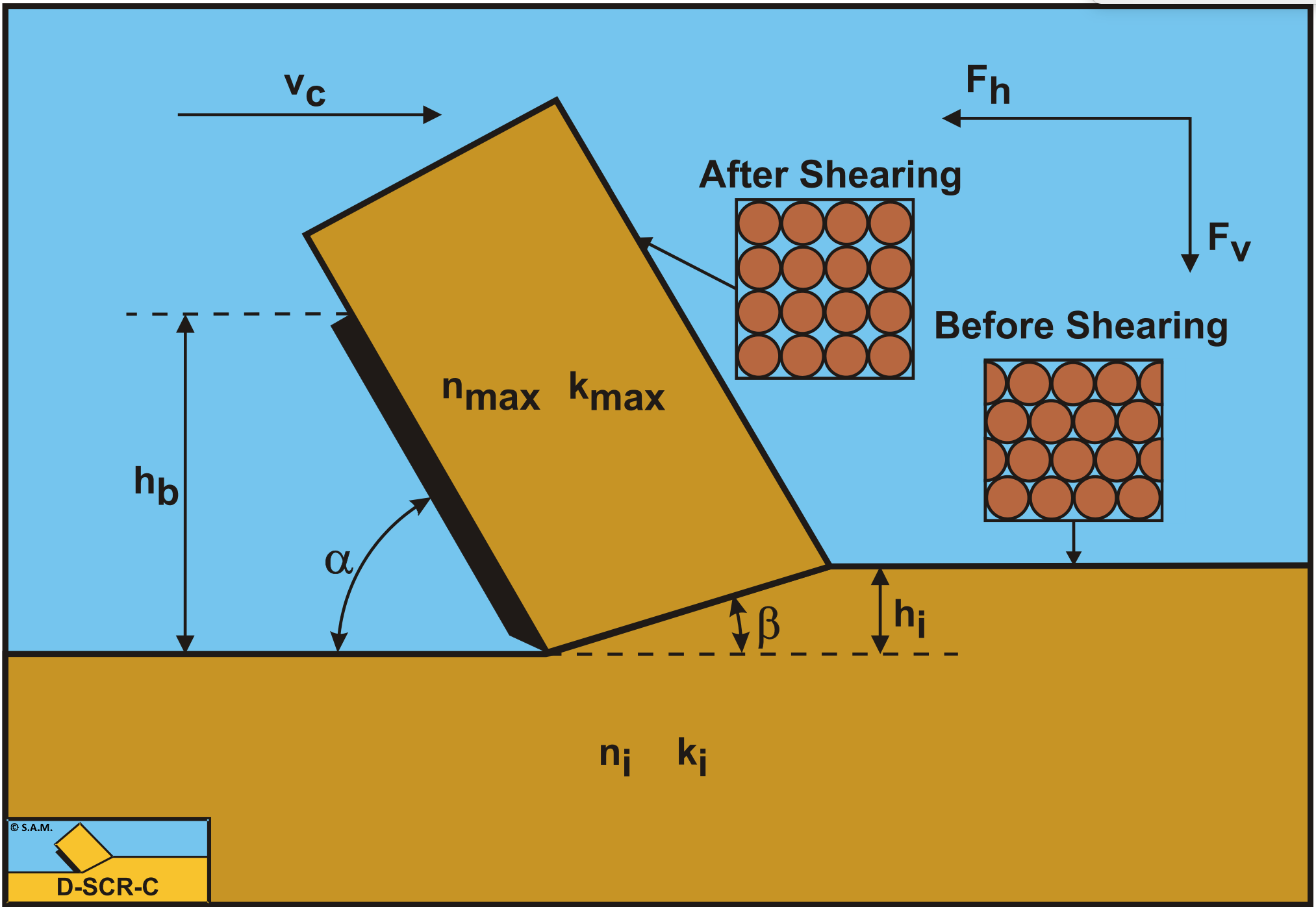
\(\newcommand{\avec}{\mathbf a}\) \(\newcommand{\bvec}{\mathbf b}\) \(\newcommand{\cvec}{\mathbf c}\) \(\newcommand{\dvec}{\mathbf d}\) \(\newcommand{\dtil}{\widetilde{\mathbf d}}\) \(\newcommand{\evec}{\mathbf e}\) \(\newcommand{\fvec}{\mathbf f}\) \(\newcommand{\nvec}{\mathbf n}\) \(\newcommand{\pvec}{\mathbf p}\) \(\newcommand{\qvec}{\mathbf q}\) \(\newcommand{\svec}{\mathbf s}\) \(\newcommand{\tvec}{\mathbf t}\) \(\newcommand{\uvec}{\mathbf u}\) \(\newcommand{\vvec}{\mathbf v}\) \(\newcommand{\wvec}{\mathbf w}\) \(\newcommand{\xvec}{\mathbf x}\) \(\newcommand{\yvec}{\mathbf y}\) \(\newcommand{\zvec}{\mathbf z}\) \(\newcommand{\rvec}{\mathbf r}\) \(\newcommand{\mvec}{\mathbf m}\) \(\newcommand{\zerovec}{\mathbf 0}\) \(\newcommand{\onevec}{\mathbf 1}\) \(\newcommand{\real}{\mathbb R}\) \(\newcommand{\twovec}[2]{\left[\begin{array}{r}#1 \\ #2 \end{array}\right]}\) \(\newcommand{\ctwovec}[2]{\left[\begin{array}{c}#1 \\ #2 \end{array}\right]}\) \(\newcommand{\threevec}[3]{\left[\begin{array}{r}#1 \\ #2 \\ #3 \end{array}\right]}\) \(\newcommand{\cthreevec}[3]{\left[\begin{array}{c}#1 \\ #2 \\ #3 \end{array}\right]}\) \(\newcommand{\fourvec}[4]{\left[\begin{array}{r}#1 \\ #2 \\ #3 \\ #4 \end{array}\right]}\) \(\newcommand{\cfourvec}[4]{\left[\begin{array}{c}#1 \\ #2 \\ #3 \\ #4 \end{array}\right]}\) \(\newcommand{\fivevec}[5]{\left[\begin{array}{r}#1 \\ #2 \\ #3 \\ #4 \\ #5 \\ \end{array}\right]}\) \(\newcommand{\cfivevec}[5]{\left[\begin{array}{c}#1 \\ #2 \\ #3 \\ #4 \\ #5 \\ \end{array}\right]}\) \(\newcommand{\mattwo}[4]{\left[\begin{array}{rr}#1 \amp #2 \\ #3 \amp #4 \\ \end{array}\right]}\) \(\newcommand{\laspan}[1]{\text{Span}\{#1\}}\) \(\newcommand{\bcal}{\cal B}\) \(\newcommand{\ccal}{\cal C}\) \(\newcommand{\scal}{\cal S}\) \(\newcommand{\wcal}{\cal W}\) \(\newcommand{\ecal}{\cal E}\) \(\newcommand{\coords}[2]{\left\{#1\right\}_{#2}}\) \(\newcommand{\gray}[1]{\color{gray}{#1}}\) \(\newcommand{\lgray}[1]{\color{lightgray}{#1}}\) \(\newcommand{\rank}{\operatorname{rank}}\) \(\newcommand{\row}{\text{Row}}\) \(\newcommand{\col}{\text{Col}}\) \(\renewcommand{\row}{\text{Row}}\) \(\newcommand{\nul}{\text{Nul}}\) \(\newcommand{\var}{\text{Var}}\) \(\newcommand{\corr}{\text{corr}}\) \(\newcommand{\len}[1]{\left|#1\right|}\) \(\newcommand{\bbar}{\overline{\bvec}}\) \(\newcommand{\bhat}{\widehat{\bvec}}\) \(\newcommand{\bperp}{\bvec^\perp}\) \(\newcommand{\xhat}{\widehat{\xvec}}\) \(\newcommand{\vhat}{\widehat{\vvec}}\) \(\newcommand{\uhat}{\widehat{\uvec}}\) \(\newcommand{\what}{\widehat{\wvec}}\) \(\newcommand{\Sighat}{\widehat{\Sigma}}\) \(\newcommand{\lt}{<}\) \(\newcommand{\gt}{>}\) \(\newcommand{\amp}{&}\) \(\definecolor{fillinmathshade}{gray}{0.9}\)The cutting process can be modeled as a two-dimensional process, in which a straight blade cuts a small layer of sand (Figure 6-7). The sand is deformed in the shear zone, also called deformation zone or dilatancy zone. During this deformation the volume of the sand changes as a result of the shear stresses in the shear zone. In soil mechanics this phenomenon is called dilatancy. In hard packed sand the pore volume is increased as a result of the shear stresses in the deformation zone. This increase in the pore volume is thought to be concentrated in the deformation zone, with the deformation zone modeled as a straight line. Water has to flow to the deformation zone to fill up the increase of the pore volume in this zone. As a result of this water flow the grain stresses increase and the water pressures decrease. Therefore there are water under-pressures.
This implies that the forces necessary for cutting hard packed sand under water will be determined for an important part by the dilatancy properties of the sand. At low cutting velocities these cutting forces are also determined by the gravity, the cohesion and the adhesion for as far as these last two soil mechanical parameters are present in the sand. Is the cutting at high velocities, then the inertia forces will have an important part in the total cutting forces especially in dry sand.
If the cutting process is assumed to be stationary, the water flow through the pores of the sand can be described in a blade motions related coordinate system. The determination of the water under-pressures in the sand around the blade is then limited to a mixed boundary conditions problem. The potential theory can be used to solve this problem. For the determination of the water under-pressures it is necessary to have a proper formulation of the boundary condition in the shear zone. Miedema (1984B) derived the basic equation for this boundary condition.
In (1985A) and (1985B) a more extensive derivation is published by Miedema. If it is assumed that no deformations take place outside the deformation zone, then the following equation applies for the sand package around the blade:
\[\ \left|\frac{\partial^{2} \mathrm{p}}{\partial \mathrm{x}^{2}}\right|+\left|\frac{\partial^{2} \mathrm{p}}{\partial \mathrm{y}^{2}}\right|=\mathrm{0}\tag{6-18}\]
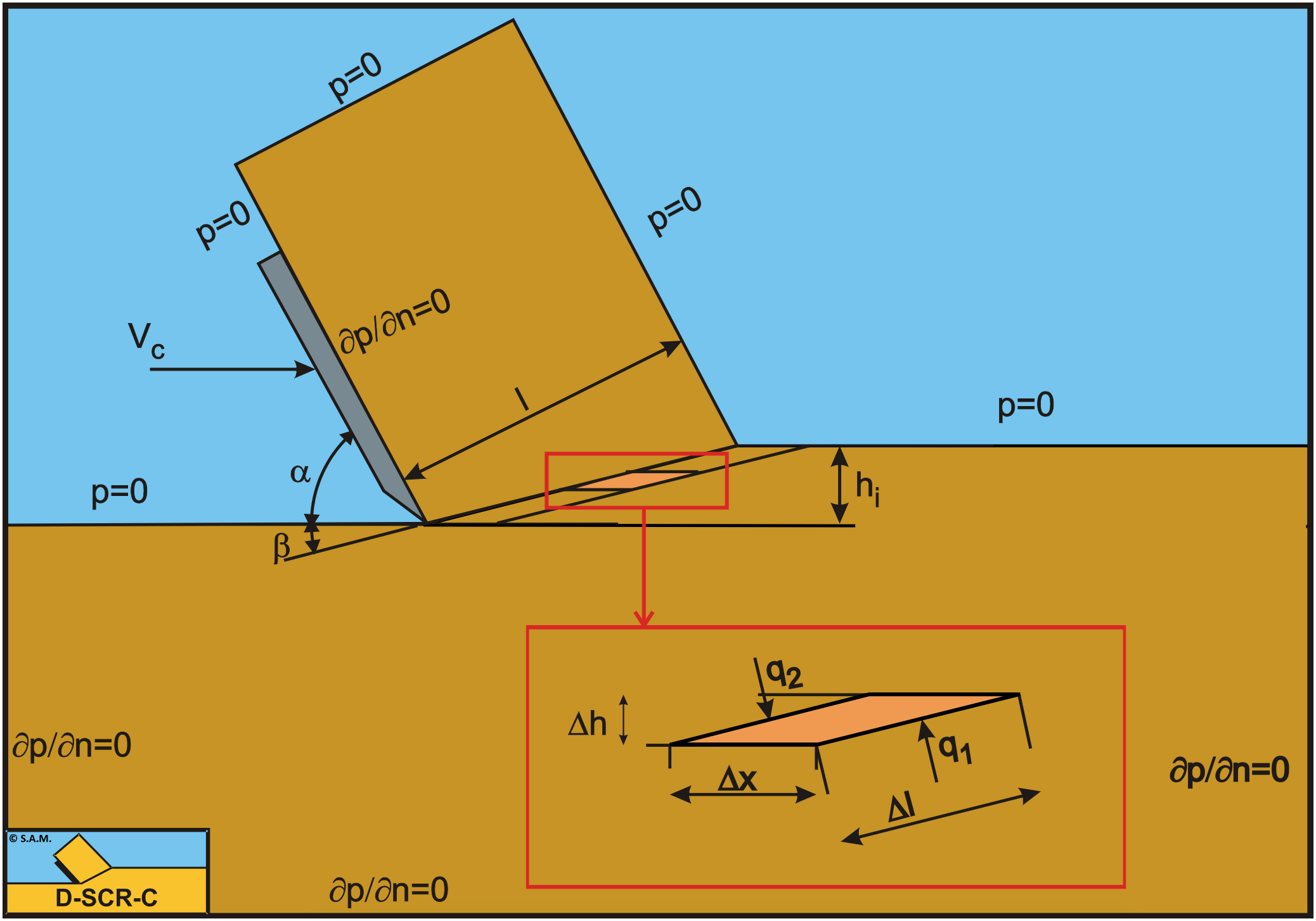
The boundary condition is in fact a specific flow rate (Figure 6-8) that can be determined with the following hypothesis. For a sand element in the deformation zone, the increase in the pore volume per unit of blade length is:
\[\ \Delta \mathrm{V}=\varepsilon \cdot \Delta \mathrm{A}=\varepsilon \cdot \Delta \mathrm{x} \cdot \Delta \mathrm{h}_{\mathrm{i}}=\varepsilon \cdot \Delta \mathrm{x} \cdot \Delta \mathrm{l} \cdot \sin (\beta)\tag{6-19}\]
\[\ \varepsilon=\frac{\mathrm{n}_{\mathrm{m a x}}-\mathrm{n}_{\mathrm{i}}}{\mathrm{1}-\mathrm{n}_{\mathrm{m a x}}}\tag{6-20}\]
It should be noted that in this book the symbol ε is used for the dilatation, while in previous publications the symbol e is often used. This is to avoid confusion with the symbol e for the void ratio.
For the residual pore percentage nmax is chosen on the basis of the ability to explain the water under-pressures, measured in laboratory tests. The volume flow rate flowing to the sand element is equal to:
\[\ \Delta \mathrm{Q}=\frac{\partial \mathrm{V}}{\partial \mathrm{t}}=\varepsilon \cdot \frac{\partial \mathrm{x}}{\partial \mathrm{t}} \cdot \Delta \mathrm{l} \cdot \sin (\beta)=\varepsilon \cdot \mathrm{v}_{\mathrm{c}} \cdot \Delta \mathrm{l} \cdot \sin (\beta)\tag{6-21}\]
With the aid of Darcy's law the next differential equation can be derived for the specific flow rate perpendicular to the deformation zone:
\[\ \mathrm{q}=\frac{\partial \mathrm{Q}}{\partial \mathrm{l}}=\mathrm{q}_{1}+\mathrm{q}_{2}=\frac{\mathrm{k}_{\mathrm{i}}}{\rho_{\mathrm{w}} \cdot \mathrm{g}} \cdot\left|\frac{\partial \mathrm{p}}{\partial \mathrm{n}}\right|_{\mathrm{1}}+\frac{\mathrm{k}_{\mathrm{m} \mathrm{a x}}}{\rho_{\mathrm{w}} \cdot \mathrm{g}} \cdot\left|\frac{\partial \mathrm{p}}{\partial \mathrm{n}}\right|_{2}=\varepsilon \cdot \mathrm{v}_{\mathrm{c}} \cdot \sin (\beta)\tag{6-22}\]
The partial derivative \(\ \partial_\mathrm{p}/\partial_\mathrm{n} \) is the derivative of the water under-pressures perpendicular on the boundary of the area, in which the water under-pressures are calculated (in this case the deformation zone). The boundary conditions on the other boundaries of this area are indicated in Figure 6-8. A hydrostatic pressure distribution is assumed on the boundaries between sand and water. This pressure distribution equals zero in the calculation of the water under-pressures, if the height difference over the blade is neglected.
The boundaries that form the edges in the sand package are assumed to be impenetrable. Making equation (6-22) dimensionless is similar to that of the breach equation of Meijer and van Os (1976). In the breach problem the length dimensions are normalized by dividing them by the breach height, while in the cutting of sand they are normalized by dividing them by the cut layer thickness.
Equation (6-22) in normalized format:
\[\ \frac{\mathrm{k}_{\mathrm{i}}}{\mathrm{k}_{\mathrm{m a x}}} \cdot\left|\frac{\partial \mathrm{p}}{\partial \mathrm{n}^{\prime}}\right|_{\mathrm{1}}+\left|\frac{\partial \mathrm{p}}{\partial \mathrm{n}^{\prime}}\right|_{\mathrm{2}}=\frac{\rho_{\mathrm{w}} \cdot \mathrm{g} \cdot \mathrm{v}_{\mathrm{c}} \cdot \varepsilon \cdot \mathrm{h}_{\mathrm{i}} \cdot \sin (\beta)}{\mathrm{k}_{\mathrm{m a x}}} \quad$ with: $\quad \mathrm{n}^{\prime}=\frac{\mathrm{n}}{\mathrm{h}_{\mathrm{i}}}\tag{6-23}\]
This equation is made dimensionless with:
\[\ \left|\frac{\partial \mathrm{p}}{\partial \mathrm{n}}\right|^{\prime}=\frac{\left|\frac{\partial \mathrm{p}}{\partial \mathrm{n}^{\prime}}\right|}{\rho_{\mathrm{w}} \cdot \mathrm{g} \cdot \mathrm{v}_{\mathrm{c}} \cdot \varepsilon \cdot \mathrm{h}_{\mathrm{i}} / \mathrm{k}_{\mathrm{m a x}}}\tag{6-24}\]
The accent indicates that a certain variable or partial derivative is dimensionless. The next dimensionless equation is now valid as a boundary condition in the deformation zone:
\[\ \frac{\mathrm{k}_{\mathrm{i}}}{\mathrm{k}_{\mathrm{m a x}}} \cdot\left|\frac{\partial \mathrm{p}}{\partial \mathrm{n}}\right|_{\mathrm{1}}^{\prime}+\left|\frac{\partial \mathrm{p}}{\partial \mathrm{n}}\right|_{\mathrm{2}}=\sin (\beta)\tag{6-25}\]
The storage equation also has to be made dimensionless, which results in the next equation:
\[\ \left|\frac{\partial^{2} \mathrm{p}}{\partial \mathrm{x}^{2}}\right|^{\prime}+\left|\frac{\partial^{2} \mathrm{p}}{\partial \mathrm{y}^{2}}\right|^{\prime}=\mathrm{0}\tag{6-26}\]
Because this equation equals zero, it is similar to equation (6-18). The water under-pressures distribution in the sand package can now be determined using the storage equation and the boundary conditions. Because the calculation of the water under-pressures is dimensionless the next transformation has to be performed to determine the real water under-pressures. The real water under-pressures can be determined by integrating the derivative of the water under-pressures in the direction of a flow line, along a flow line, so:
\[\ \mathrm{P}_{\mathrm{calc}}=\int_{\mathrm{s}^{\prime}}\left|\frac{\partial \mathrm{p}}{\partial \mathrm{s}}\right|^{\prime} \cdot \mathrm{d s}^{\prime}\tag{6-27}\]
This is illustrated in Figure 6-9. Using equation (6-30) this is written as:
\[\ \mathrm{P}_{\text {real }}=\int_{\mathrm{s}}\left|\frac{\partial \mathrm{p}}{\partial \mathrm{s}}\right| \cdot \mathrm{d s}=\int_{\mathrm{s}^{\prime}} \frac{\rho_{\mathrm{w}} \cdot \mathrm{g} \cdot \mathrm{v}_{\mathrm{c}} \cdot \mathrm{\varepsilon} \cdot \mathrm{h}_{\mathrm{i}}}{\mathrm{k}_{\mathrm{m a x}}} \cdot\left|\frac{\partial \mathrm{p}}{\partial \mathrm{s}}\right|^{\prime} \cdot \mathrm{d} \mathrm{s}^{\prime} \quad\text{ with: }\quad \mathrm{s}^{\prime}=\frac{\mathrm{s}}{\mathrm{h}_{\mathrm{i}}}\tag{6-28}\]
This gives the next relation between the real emerging water under-pressures and the calculated water under-pressures:
\[\ \mathrm{P}_{\text {real }}=\frac{\rho_{\mathrm{w}} \cdot \mathrm{g} \cdot \mathrm{v}_{\mathrm{c}} \cdot \boldsymbol{\varepsilon} \cdot \mathrm{h}_{\mathrm{i}}}{\mathrm{k}_{\mathrm{m a x}}} \cdot \mathrm{P}_{\mathrm{c a l c}}\tag{6-29}\]
To be independent of the ratio between the initial permeability ki and the maximum permeability kmax , kmax has to be replaced with the weighted average permeability km before making the measured water under-pressures dimensionless.