Shear Stress
- Page ID
- 615
\( \newcommand{\vecs}[1]{\overset { \scriptstyle \rightharpoonup} {\mathbf{#1}} } \)
\( \newcommand{\vecd}[1]{\overset{-\!-\!\rightharpoonup}{\vphantom{a}\smash {#1}}} \)
\( \newcommand{\dsum}{\displaystyle\sum\limits} \)
\( \newcommand{\dint}{\displaystyle\int\limits} \)
\( \newcommand{\dlim}{\displaystyle\lim\limits} \)
\( \newcommand{\id}{\mathrm{id}}\) \( \newcommand{\Span}{\mathrm{span}}\)
( \newcommand{\kernel}{\mathrm{null}\,}\) \( \newcommand{\range}{\mathrm{range}\,}\)
\( \newcommand{\RealPart}{\mathrm{Re}}\) \( \newcommand{\ImaginaryPart}{\mathrm{Im}}\)
\( \newcommand{\Argument}{\mathrm{Arg}}\) \( \newcommand{\norm}[1]{\| #1 \|}\)
\( \newcommand{\inner}[2]{\langle #1, #2 \rangle}\)
\( \newcommand{\Span}{\mathrm{span}}\)
\( \newcommand{\id}{\mathrm{id}}\)
\( \newcommand{\Span}{\mathrm{span}}\)
\( \newcommand{\kernel}{\mathrm{null}\,}\)
\( \newcommand{\range}{\mathrm{range}\,}\)
\( \newcommand{\RealPart}{\mathrm{Re}}\)
\( \newcommand{\ImaginaryPart}{\mathrm{Im}}\)
\( \newcommand{\Argument}{\mathrm{Arg}}\)
\( \newcommand{\norm}[1]{\| #1 \|}\)
\( \newcommand{\inner}[2]{\langle #1, #2 \rangle}\)
\( \newcommand{\Span}{\mathrm{span}}\) \( \newcommand{\AA}{\unicode[.8,0]{x212B}}\)
\( \newcommand{\vectorA}[1]{\vec{#1}} % arrow\)
\( \newcommand{\vectorAt}[1]{\vec{\text{#1}}} % arrow\)
\( \newcommand{\vectorB}[1]{\overset { \scriptstyle \rightharpoonup} {\mathbf{#1}} } \)
\( \newcommand{\vectorC}[1]{\textbf{#1}} \)
\( \newcommand{\vectorD}[1]{\overrightarrow{#1}} \)
\( \newcommand{\vectorDt}[1]{\overrightarrow{\text{#1}}} \)
\( \newcommand{\vectE}[1]{\overset{-\!-\!\rightharpoonup}{\vphantom{a}\smash{\mathbf {#1}}}} \)
\( \newcommand{\vecs}[1]{\overset { \scriptstyle \rightharpoonup} {\mathbf{#1}} } \)
\(\newcommand{\longvect}{\overrightarrow}\)
\( \newcommand{\vecd}[1]{\overset{-\!-\!\rightharpoonup}{\vphantom{a}\smash {#1}}} \)
\(\newcommand{\avec}{\mathbf a}\) \(\newcommand{\bvec}{\mathbf b}\) \(\newcommand{\cvec}{\mathbf c}\) \(\newcommand{\dvec}{\mathbf d}\) \(\newcommand{\dtil}{\widetilde{\mathbf d}}\) \(\newcommand{\evec}{\mathbf e}\) \(\newcommand{\fvec}{\mathbf f}\) \(\newcommand{\nvec}{\mathbf n}\) \(\newcommand{\pvec}{\mathbf p}\) \(\newcommand{\qvec}{\mathbf q}\) \(\newcommand{\svec}{\mathbf s}\) \(\newcommand{\tvec}{\mathbf t}\) \(\newcommand{\uvec}{\mathbf u}\) \(\newcommand{\vvec}{\mathbf v}\) \(\newcommand{\wvec}{\mathbf w}\) \(\newcommand{\xvec}{\mathbf x}\) \(\newcommand{\yvec}{\mathbf y}\) \(\newcommand{\zvec}{\mathbf z}\) \(\newcommand{\rvec}{\mathbf r}\) \(\newcommand{\mvec}{\mathbf m}\) \(\newcommand{\zerovec}{\mathbf 0}\) \(\newcommand{\onevec}{\mathbf 1}\) \(\newcommand{\real}{\mathbb R}\) \(\newcommand{\twovec}[2]{\left[\begin{array}{r}#1 \\ #2 \end{array}\right]}\) \(\newcommand{\ctwovec}[2]{\left[\begin{array}{c}#1 \\ #2 \end{array}\right]}\) \(\newcommand{\threevec}[3]{\left[\begin{array}{r}#1 \\ #2 \\ #3 \end{array}\right]}\) \(\newcommand{\cthreevec}[3]{\left[\begin{array}{c}#1 \\ #2 \\ #3 \end{array}\right]}\) \(\newcommand{\fourvec}[4]{\left[\begin{array}{r}#1 \\ #2 \\ #3 \\ #4 \end{array}\right]}\) \(\newcommand{\cfourvec}[4]{\left[\begin{array}{c}#1 \\ #2 \\ #3 \\ #4 \end{array}\right]}\) \(\newcommand{\fivevec}[5]{\left[\begin{array}{r}#1 \\ #2 \\ #3 \\ #4 \\ #5 \\ \end{array}\right]}\) \(\newcommand{\cfivevec}[5]{\left[\begin{array}{c}#1 \\ #2 \\ #3 \\ #4 \\ #5 \\ \end{array}\right]}\) \(\newcommand{\mattwo}[4]{\left[\begin{array}{rr}#1 \amp #2 \\ #3 \amp #4 \\ \end{array}\right]}\) \(\newcommand{\laspan}[1]{\text{Span}\{#1\}}\) \(\newcommand{\bcal}{\cal B}\) \(\newcommand{\ccal}{\cal C}\) \(\newcommand{\scal}{\cal S}\) \(\newcommand{\wcal}{\cal W}\) \(\newcommand{\ecal}{\cal E}\) \(\newcommand{\coords}[2]{\left\{#1\right\}_{#2}}\) \(\newcommand{\gray}[1]{\color{gray}{#1}}\) \(\newcommand{\lgray}[1]{\color{lightgray}{#1}}\) \(\newcommand{\rank}{\operatorname{rank}}\) \(\newcommand{\row}{\text{Row}}\) \(\newcommand{\col}{\text{Col}}\) \(\renewcommand{\row}{\text{Row}}\) \(\newcommand{\nul}{\text{Nul}}\) \(\newcommand{\var}{\text{Var}}\) \(\newcommand{\corr}{\text{corr}}\) \(\newcommand{\len}[1]{\left|#1\right|}\) \(\newcommand{\bbar}{\overline{\bvec}}\) \(\newcommand{\bhat}{\widehat{\bvec}}\) \(\newcommand{\bperp}{\bvec^\perp}\) \(\newcommand{\xhat}{\widehat{\xvec}}\) \(\newcommand{\vhat}{\widehat{\vvec}}\) \(\newcommand{\uhat}{\widehat{\uvec}}\) \(\newcommand{\what}{\widehat{\wvec}}\) \(\newcommand{\Sighat}{\widehat{\Sigma}}\) \(\newcommand{\lt}{<}\) \(\newcommand{\gt}{>}\) \(\newcommand{\amp}{&}\) \(\definecolor{fillinmathshade}{gray}{0.9}\)The shear stress is part of the pressure tensor. However, here, and many parts of the book, it will be treated as a separate issue. In solid mechanics, the shear stress is considered as the ratio of the force acting on area in the direction of the forces perpendicular to area. Different from solid, fluid cannot pull directly but through a solid surface. Consider liquid that undergoes a shear stress between a short distance of two plates as shown in Figure 1.3.

Figure 1.3: Schematics to describe the shear stress in fluid mechanics.
The upper plate velocity generally will be
\[U = \ff(A, F, h)\]
Where \(A\) is the area, the \(F\) denotes the force, and \(h\) is the distance between the plates. From solid mechanics study, it was shown that when the force per area increases, the velocity of the plate increases also. Experiments show that the increase of height will increase the velocity up to a certain range. Consider moving the plate with a zero lubricant \((h \sim 0)\) (results in large force) or a large amount of lubricant (smaller force). In this discussion, the aim is to develop differential equation, thus the small distance analysis is applicable. For cases where the dependency is linear, the following can be written \[U \propto \dfrac{h F}{A} \]
Equations qref{intro:eq:Upropto} can be rearranged to be
\[U h \propto \dfrac{F}{A} \]
Shear stress was defined as
\[T_{xy} = \dfrac{F}{A}\]
The index x represent the ``direction of the shear stress while the y represent the direction of the area(perpendicular to the area). From equations qref{intro:eq:UproptoA} and qref{intro:eq:tauDef} it follows that ratio of the velocity to height is proportional to shear stress. Hence, applying the coefficient to obtain a new equality as
\[T_{xy} = \mu \dfrac{U}{h}\]
Where \mu is called the absolute viscosity or dynamic viscosity which will be discussed later in this chapter in a great length.

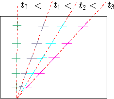
Fig. 1.4 The deformation of fluid due to shear stress as progression of time.
In steady state, the distance the upper plate moves after small amount of time, \delta t is
\[dll = U \delta t \]
From Figure 1.4 it can be noticed that for a small angle, \(\delta\beta \cong \sin\beta\), the regular approximation provides
\[dll = U \delta t = h\delta\beta\]
From equation qref{intro:eq:dUdx} it follows that
\[U=h\dfrac{\delta\beta}{\delta t}\]
Combining equation qref{intro:eq:dbdt} with equation qref{intro:eq:shearS} yields
\[T_{xy} = \mu\dfrac{\delta\beta}{\delta t}\]
If the velocity profile is linear between the plate (it will be shown later that it is consistent with derivations of velocity), then it can be written for small a angel that
\[\dfrac{\delta \beta}{\delta t} = \dfrac{dU}{dy}\]
Materials which obey equation qref{intro:eq:tau_dbdt} referred to as Newtonian fluid. For this kind of substance
\[T_{xy} = \mu\dfrac{dU}{dy}\]
Newtonian fluids are fluids which the ratio is constant. Many fluids fall into this category such as air, water etc. This approximation is appropriate for many other fluids but only within some ranges. Equation qref{intro:eq:dbdt} can be interpreted as momentum in the \x direction transferred into the \y direction. Thus, the viscosity is the resistance to the flow (flux) or the movement. The property of viscosity, which is exhibited by all fluids, is due to the existence of cohesion and interaction between fluid molecules. These cohesion and interactions hamper the flux in y–direction. Some referred to shear stress as viscous flux of x–momentum in the y–direction. The units of shear stress are the same as flux per time as following
\[\dfrac{F}{A}\left\dfrac{kg m}{sec^2}\dfrac{1}{m^2}\right = \dfrac{mU}{A}\left\dfrac{kg}{sec}\dfrac{m}{sec}\dfrac{1}{m^2}\righttag\]
τxy=FA(5)
τxy=FA(5)jUh∝FA(4)
Thus, the notation of \(T_{xy}\) is easier to understand and visualize. In fact, this interpretation is more suitable to explain the molecular mechanism of the viscosity. The units of absolute viscosity are \([N sec / m^2]\).


