1.5.4: Estimation of the Viscosity
- Page ID
- 626
The absolute viscosity of many fluids relatively doesn't change with the pressure but very sensitive to temperature. For isothermal flow, the viscosity can be considered constant in many cases. The variations of air and water as a function of the temperature at atmospheric pressure are plotted in Figures 1.8 and 1.9.
Some common materials (pure and mixture) have expressions that provide an estimate. For many gases, Sutherland's equation is used and according to the literature, provides reasonable of \(-40°C\) to \(1600°C\). \[\mu = \mu_{0} \frac{0.555 T_{i0} + Suth}{0.555 T_{in} + Suth} (\frac{T}{T_0})^\frac{3}{2}\]
Where
\(\mu\) viscosity at input temperature, T
\(\mu_{0}\) reference viscosity at reference temperature, \(T_{i0})
\(T_{in}\) input temperature in degrees Kelvin
\(T_{i0}\) reference temperature in degrees Kelvin
\(Suth\) Sutherland's constant (presented in Table 1.1)
Example 1.3
Calculate the viscosity of air at 800K based on Sutherland's equation. Use the data provide in Table 1.1.
Solution 1.3
Applying the constants from Suthelnd's table provides
\[ \mu = 0.00001827 \times \dfrac{ 0.555\times524.07+120}{0.555\times800+120} \times \left( \dfrac{800}{524.07}\right)^{\dfrac{3}{2}} \ \sim 2.51\,{10}^{-5} \left[\dfrac{N\, sec}{m^2}\right] \]
The observed viscosity is about \(\sim 3.7{10}^{-5}\left[\dfrac{N\, sec}{m^2}\right]\).
Table 1.2 Viscosity of selected gases.
| Substance | Chemical formula | Temperature, \(T\,[^{\circ}C]\) | Viscosity, \(\left[\dfrac{N\, sec}{m^2} \right]\) |
| \(i-C_4\,H_{10}\) | 23 | 0.0000076 | |
| \(CH_4\) | 20 | 0.0000109 | |
| Oxygen | \(O_2\) | 20 | 0.0000203 |
| Mercury Vapor | \(Hg\) | 380 | 0.0000654 |
Table 1.3 Viscosity of selected liquids.
| Substance | Chemical formula | Temperature, \(T\,[^{\circ}C]\) | Viscosity, \(\left[\dfrac{N\, sec}{m^2} \right]\) |
| \((C_2H_5)O\) | 20 | 0.000245 | |
| \(C_6H_6\) | 20 | 0.000647 | |
| \(Br_2\) | 26 | 0.000946 | |
| \(C_2H_5OH\) | 20 | 0.001194 | |
| \(Hg\) | 25 | 0.001547 | |
| \(H_2SO_4\) | 25 | 0.01915 | |
| Olive Oil | 25 | 0.084 | |
| Castor Oil | 25 | 0.986 | |
| Clucuse | 25 | 5-20 | |
| Corn Oil | 20 | 0.072 | |
| SAE 30 | - | 0.15-0.200 | |
| SAE 50 | \(\sim25^{\circ}C\) | 0.54 | |
| SAE 70 | \(\sim25^{\circ}C\) | 1.6 | |
| Ketchup | \(\sim20^{\circ}C\) | 0,05 | |
| Ketchup | \(\sim25^{\circ}C\) | 0,098 | |
| Benzene | \(\sim20^{\circ}C\) | 0.000652 | |
| Firm glass | - | \(\sim 1\times10^7\) | |
| Glycerol | 20 | 1.069 |
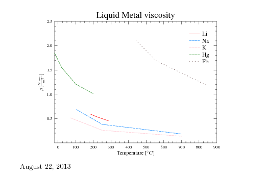
Fig. 1.10. Liquid metals' viscosity as a function of the temperature.
Liquid Metals
Liquid metal can be considered as a Newtonian fluid for many applications. Furthermore, many aluminum alloys are behaving as a Newtonian liquid until the first solidification appears (assuming steady state thermodynamics properties). Even when there is a solidification (mushy zone), the metal behavior can be estimated as a Newtonian material (further reading can be done in this author's book ``Fundamentals of Die Casting Design''). Figure 1.10 exhibits several liquid metals (from The Reactor Handbook, Vol. Atomic Energy Commission AECD-3646 U.S. Government Printing Office, Washington D.C. May 1995 p. 258.)
The General Viscosity Graphs
In case ``ordinary'' fluids where information is limit, Hougen et al suggested to use graph similar to compressibility chart. In this graph, if one point is well documented, other points can be estimated. Furthermore, this graph also shows the trends. In Figure 1.11 the relative viscosity \(\mu_{r} = \mu / \mu_{c}\) is plotted as a function of relative temperature, \(T_{r}\). \(\mu_{c}\) is the viscosity at critical condition and \(\mu\) is the viscosity at any given condition. The lines of constant relative pressure \(P_{r} = P / P_{c}\) are drawn. The lower pressure is, for practical purpose, \(\sim1[bar]\).
Table 1.3 Viscosity of selected liquids.
| Chemical component | Molecular Weight | \(T_c\)[K] | \(P_c\)[Bar] | \(\mu_c\)\(\left[\dfrac{N\,sec}{m^2}\right]\) |
| \(H_2\) | 2.016 | 33.3 | 12.9696 | 3.47 |
| \(He\) | 4.003 | 5.26 | 2.289945 | 2.54 |
| \(Ne\) | 20.183 | 44.5 | 27.256425 | 15.6 |
| \(Ar\) | 39.944 | 151 | 48.636 | 26.4 |
| \(Xe\) | 131.3 | 289.8 | 58.7685 | 49. |
| Air "mixed'' | 28.97 | 132 | 36.8823 | 19.3 |
| \(CO_2\) | 44.01 | 304.2 | 73.865925 | 19.0 |
| \(O_2\) | 32.00 | 154.4 | 50.358525 | 18.0 |
| \(C_2H_6\) | 30.07 | 305.4 | 48.83865 | 21.0 |
| \(CH_4\) | 16.04 | 190.7 | 46.40685 | 15.9 |
| Water | 18.01528 | 647.096 K | 22.064 [MPa] | ∼ 11. |
The critical pressure can be evaluated in the following three ways. The simplest way is by obtaining the data from Table 1.4 or similar information. The second way, if the information is available and is close enough to the critical point, then the critical viscosity is obtained as \[\mu_{c} = \frac{\mu}{\mu_{r}}\] The third way, when none is available, is by utilizing the following approximation \[\mu_{c} = \sqrt{MT_{c}}v_{c}^{2/3}\] Where ___vc with sim hat___ is the critical molecular volume and \(M\) is molecular weight. Or \[\mu_{c} = \sqrt{M}P_{c}^{2/3}T_{c}^{-1/6}\] Calculate the reduced pressure and the reduced temperature and from the Figure 1.11 obtain the reduced viscosity.
Example 1.4
Estimate the viscosity of oxygen, \(O_2\) at \(100^{\circ}C\) and 20[Bar].
Solution 1.4
\(P_c = 50.35[Bar]\,\) \(T_c=154.4\) and therefore \(\mu_c=18 \left[ \dfrac{N\,sec}{m^2}\right]\) The value of the reduced temperature is
\[\left[ \dfrac{N\,sec}{m^2}\right] \]
\[P_r \sim \dfrac{20}{50.35} \sim 0.4 \] From Figure 1.11 it can be obtained \(\mu_r\sim 1.2\) and the predicted viscosity is
\[\mu = \mu_c \, \overbrace{\left( \dfrac{\mu}{\mu_c}\right)}
^{Table } = 18 \times 1.2 = 21.6[N sec/m^2] \]
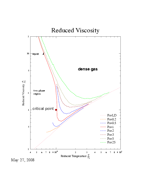
Fig. 1.11. Reduced viscosity as a function of the reduced temperature.
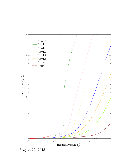
Fig. 1.12. Reduced viscosity as a function of the reduced temperature.
Viscosity of Mixtures
In general the viscosity of liquid mixture has to be evaluated experimentally. Even for homogeneous mixture, there isn't silver bullet to estimate the viscosity. In this book, only the mixture of low density gases is discussed for analytical expression. For most cases, the following Wilke's correlation for gas at low density provides a result in a reasonable range. \[\mu_{mix} = \sum_{i=1}^n \frac{x_{i}\mu_{i}}{\sum_{j=1}^n x_{i}\phi_{ij}}\] where \(\phi_{ij}\) is defined as \[\phi_{ij} = \frac{1}{\sqrt{8}}\sqrt{1+\frac{M_i}{M_j}}(1+\sqrt{\frac{mu_i}{mu_j}}{\frac{M_j}{M_i})^2\)
Here,
\(n\) the number of the chemical components in the mixture
\(x_{i}\) is the mole fraction of component \(i\)
\mu_{i} the viscosity of component \(i\)
The subscript \(i\) should be used for the \(j\) index.
The dimensionless parameter \(\phi_{ij}\)
is equal to one when \(i=j\). The mixture viscosity is highly nonlinear function of the fractions of the components.
Example 1.5
Calculate the viscosity of a mixture (air) made of 20% oxygen, \(O_2\) and 80% nitrogen \(N_2\) for the temperature of \(20^{\circ}C\).
Solution 1.5
The following table summarizes the known details
Table summary 1.
| Component | Molecular Weight, \(M\) | Fraction, \(x\) | Viscosity, \(\mu\) |
| \(O_2\) | 32. | 0.2 | 0.0000203 |
| \(N_2\) | 28. | 0.8 | 0.00001754 |
Table summary 2.
| i | j | \(M_i/M_j\) | \(\mu_i/\mu_j\) | \(\Phi_{ij}\) |
| 1 | 1 | 1.0 | 1.0 | 1.0 |
| 1 | 2 | 1.143 | 1.157 | 1.0024 |
| 2 | 1 | 0.875 | .86 | 0.996 |
| 2 | 2 | 1.0 | 1.0 | 1. |
\[ \mu_{mix} \sim \dfrac{0.2\times 0.0000203}{0.2\times1.0 + 0.8\times 1.0024} + \\ \dfrac{0.8\times 0.00001754}{0.2\times0.996 + 0.8\times 1.0} \sim 0.0000181 \left[\dfrac{N\,sec}{m^2}\right] \]
The observed value is \(\sim0.0000182 \left[\dfrac{N\,sec}{m^2}\right]\).
In very low pressure, in theory, the viscosity is only a function of the temperature with a ``simple'' molecular structure. For gases with very long molecular structure or complexity structure these formulas cannot be applied. For some mixtures of two liquids it was observed that at a low shear stress, the viscosity is dominated by a liquid with high viscosity and at high shear stress to be dominated by a liquid with the low viscosity liquid. The higher viscosity is more dominate at low shear stress. Reiner and Phillippoff suggested the following formula:
\[\frac{dU_{x}}{dy} = \left(\frac{1}{\mu_{\infty} + \frac{\mu_{0} - \mu_{\infty}}{1 + (\frac{\tau_{xy}}{\tau_{s}})^2}}\right)\tau_{xy}\]
Where the term \(\mu_{\infty}\) is the experimental value at high shear stress. The term \(\mu_0\) is the experimental viscosity at shear stress approaching zero. The term \(\tau_s\) is the characteristic shear stress of the mixture. An example for values for this formula, for Molten Sulfur at temperature \(120^{\circ}C\) are \(\mu_{\infty} = 0.0215 \left({N\,sec}/{m^2}\right)\), \(\mu_{0} = 0.00105 \left({N\,sec}/{m^2}\right)\), and \(\tau_s = 0.0000073 \left({kN}/{m^2}\right)\). This equation (29) provides reasonable value only up to \(\tau = 0.001 \left({kN}/{m^2}\right)\).
Figure 1.12 can be used for a crude estimate of dense gases mixture. To estimate the viscosity of the mixture with \(n\) component Hougen and Watson's method for pseudocritial properties is adapted. In this method the following are defined as mixed critical pressure as
\[{P_c}_{mix} = \sum_{i=1}^{n} \, x_i \,{P_c}_i \]
\[{T_c}_{mix} = \sum_{i=1}^{n} \,x_i\, {T_c}_i \] and the mixed critical viscosity is
\[{\mu_c}_{mix} = \sum_{i=1}^{n} \,x_i\, {\mu_c}_i \]
Example 1.6
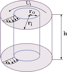
Fig. 1.13 Concentrating cylinders with the rotating inner cylinder.
of 0.101 [m] radius and the cylinders length is 0.2 [m]. It is given that a moment of 1 [\(N\times m\)] is required to maintain an angular velocity of 31.4 revolution per second (these number represent only academic question not real value of actual liquid). Estimate the liquid viscosity used between the cylinders.}
Solution 1.6
The moment or the torque is transmitted through the liquid to the outer cylinder. Control volume around the inner cylinder shows that moment is a function of the area and shear stress. The shear stress calculations can be estimated as a linear between the two concentric cylinders. The velocity at the inner cylinders surface is \[ \label{concentricCylinders:Ui} U_i = r\,\omega = 0.1\times 31.4[rad/second] = 3.14 [m/s] \] The velocity at the outer cylinder surface is zero. The velocity gradient may be assumed to be linear, hence, \[ \label{concentricCylinders:dUdr} \dfrac{dU}{dr} \cong \dfrac{0.1- 0}{0.101 - 0.1} = 100 sec^{-1} \] The used moment is \[ \label{concentricCylinders:M1} M = \overbrace{2\,\pi\,r_i\,h}^{A} \overbrace{\mu \dfrac{dU}{dr}}^{\tau} \,\overbrace{r_i}^{ll} \] or the viscosity is \[ \label{concentricCylinders:M} \mu = \dfrac{M}{ {2\,\pi\,{r_i}^2\,h} { \dfrac{dU}{dr}} } = \dfrac{1}{2\times\pi\times{0.1}^2 \times 0.2 \times 100} = \]
Example 1.7
A square block weighing 1.0 [kN] with a side surfaces area of 0.1 [\(m^2\)] slides down an incline surface with an angle of 20\0C. The surface is covered with oil film. The oil creates a distance between the block and the inclined surface of \(1\times10^{-6}[m]\). What is the speed of the block at steady state? Assuming a linear velocity profile in the oil and that the whole oil is under steady state. The viscosity of the oil is \(3 \times 10^{-5} [m^2/sec]\).
Solution 1.7
The shear stress at the surface is estimated for steady state by \[ \label{slidingBlock:shear} \tau = \mu \dfrac{dU}{dx} = 3 \times 10^{-5} \times \dfrac{U}{1\times10^{-6}} = 30 \, U \] The total fiction force is then \[ \label{slidingBlock:frictionForce} f = \tau\, A = 0.1 \times 30\,U = 3\,U \] The gravity force that acting against the friction is equal to the friction hence \[ \label{slidingBlock:solPre1} F_g = f = 3\,U\Longrightarrow U = \dfrac{m\,g\,\sin\,20^{\circ}}{3} \] Or the solution is \[ \label{slidingBlock:solPre} U = \dfrac{1\times 9.8\times\sin\,20^{\circ}}{3} \]
Example 1.8
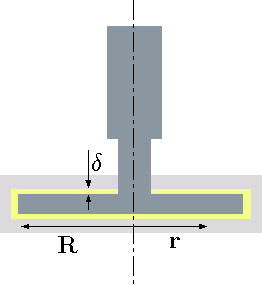
Fig. 1.14 Rotating disc in a steady state.
The edge effects can be neglected. The gap is given and equal to \(\delta\) and the rotation speed is \(\omega\). The shear stress can be assumed to be linear.}
Solution 1.8
In this cases the shear stress is a function of the radius, \(r\) and an expression has to be developed. Additionally, the differential area also increases and is a function of \(r\). The shear stress can be estimated as \[ \label{discRotating:tau} \tau \cong \mu \,\dfrac{U}{\delta} = \mu\,\dfrac{\omega \, r}{\delta} \] This torque can be integrated for the entire area as \[ \label{discRotating:F} T = \int_0^R r\, \tau \,dA = \int_0^R \overbrace{r}^{ll} \, \overbrace{\mu\, \dfrac{\omega \, r}{\delta}}^{\tau} \, \overbrace{2\,\pi\,r\,dr}^{dA} \] The results of the integration is \[ \label{discRotating:I} T = \dfrac{\pi\,\mu\,\omega\,R^4}{2\,\delta} \]


