4.2: The Hydrostatic Equation

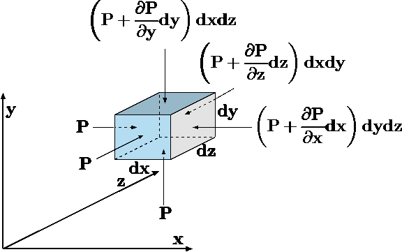
Fig 4.1. Description of a fluid element in accelerated system under body forces.

A fluid element with dimensions of \(DC\), \(dy\), and \(dz\) is motionless in the accelerated system, with acceleration, \(a\) as shown in Figure 4.1. The combination of an acceleration and the body force results in effective body force which is \[g_{G} - a = g_{eff}\] Equation 1 can be reduced and simplified for the case of zero acceleration, \(a = 0\). In these derivations, several assumptions must be made. The first assumption is that the change in the pressure is a continuous function. There is no requirement that the pressure has to be a monotonous function e.g. that pressure can increase and later decrease. The changes of the second derivative pressure are not significant compared to the first derivative \(\left(\partial{P}/\partial{n} \times dl > > \partial^{2}{P} / \partial{n^{2}}\right)\), where \(n\) is the steepest direction of the pressure derivative and \(dl\) is the infinitesimal length. This mathematical statement simply requires that the pressure can deviate in such a way that the average on infinitesimal area can be found and expressed as only one direction. The net pressure force on the faces in the \(x\) direction results in \[dF = -\left(\frac{\partial{P}}{\partial{x}}\right)dydx \hat{i}\] In the same fashion, the calculations of the three directions result in the total net pressure force as \[\sum_{surface} F = - \left(\frac{\partial{P}}{\partial{x}} \hat{i} + \frac{\partial{P}}{\partial{y}} \hat{j} + \frac{\partial{P}}{\partial{y}} \hat{k}\right)\] The term in the parentheses in equation 3 referred to in the literature as the pressure gradient (see for more explanation in the Mathematics Appendix). This mathematical operation has a geometrical interpretation. If the pressure, \(P\), was a two–dimensional height (that is only a function of \(x\) and \(y\) ) then the gradient is the steepest ascent of the height (to the valley). The second point is that the gradient is a vector (that is, it has a direction). Even though, the pressure is treated, now, as a scalar function (there no reference to the shear stress in part of the pressure) the gradient is a vector. For example, the dot product of the following is \[\hat{i} \cdot \mathbf{grad}P = \hat{i} \cdot \nabla P = \frac{\partial{P}}{\partial{x}} \] In general, if the coordinates were to ``rotate/transform'' to a new system which has a different orientation, the dot product results in \[\bar{i_{n}} \cdot \mathbf{grad}P = \bar{i_{n}} \cdot \nabla P = \frac{\partial{P}}{\partial{n}} \] where \(i_{n}\) is the unit vector in the \(n\) direction and \(\partial / \partial{n}\) is a derivative in that direction. As before, the effective gravity force is utilized in case where the gravity is the only body force and in an accelerated system. The body (element) is in rest and therefore the net force is zero \[\sum_{total} F = \sum_{surface} F + \sum_{body} F \] Hence, the utilizing the above derivations one can obtain \[- \mathbf{grad} P dx dy dz + \rho g_{eff} dx dy dz = 0\] or

Pressure Gradient

\[\mathbf{grad}P = \nabla P = \rho g_{eff} \]

Some refer to equation 8 as the Fluid Static Equation. This equation can be integrated and therefore solved. However, there are several physical implications to this equation which should be discussed and are presented here. First, a discussion on a simple condition and will continue in more challenging situations.

Contributors and Attributions

• Dr. Genick Bar-Meir. Permission is granted to copy, distribute and/or modify this document under the terms of the GNU Free Documentation License, Version 1.2 or later or Potto license.