4.7: Rayleigh–Taylor Instability

Rayleigh–Taylor instability (or RT instability) is named after Lord Rayleigh and G. I. Taylor. There are situations where a heavy liquid layer is placed over a lighter fluid layer. This situation has engineering implications in several industries. For example in die casting, liquid metal is injected in a cavity filled with air. In poor designs or other situations, some air is not evacuated and stay in small cavity on the edges of the shape to be casted. Thus, it can create a situation where the liquid metal is above the air but cannot penetrate into the cavity because of instability. This instability deals with a dense, heavy fluid that is being placed above a lighter fluid in a gravity field perpendicular to interface. Example for such systems are dense water over oil (liquid–liquid), or water over air(gas–liquid). The original Rayleigh's paper deals with the dynamics and density variations. For example, density variations according to the bulk modulus (see section 4.3.3.2) are always stable but unstable of the density is in the reversed order. Supposed that a liquid density is arbitrary function of the height. This distortion can be as a result of heavy fluid above the lighter liquid. This analysis asks the question of what happen when a small amount of liquid from the above layer enter into the lower layer? Whether this liquid continue and will grow or will it return to its original conditions? The surface tension is the opposite mechanism that will returns the liquid to its original place. This analysis is referred to the case of infinite or very large surface. The simplified case is the two different uniform densities. For example a heavy fluid density , \(\rho_{L}\), above lower fluid with lower density, \(\rho_{G}\). For perfectly straight interface, the heavy fluid will stay above the lighter fluid. If the surface will be disturbed, some of heavy liquid moves down. This disturbance can grow or returned to its original situation. This condition is determined by competing forces, the surface density, and the buoyancy forces. The fluid above the depression is in equilibrium with the sounding pressure since the material is extending to infinity. Thus, the force that acting to get the above fluid down is the buoyancy force of the fluid in the depression.

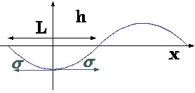
Fig. 4.48. Description of depression to explain the Rayleigh-Taylor instability.

The depression is returned to its original position if the surface forces are large enough. In that case, this situation is considered to be stable. On the other hand, if the surface forces (surface tension) are not sufficient, the situation is unstable and the heavy liquid enters into the liquid fluid zone and vice versa. As usual there is the neutral stable when the forces are equal. Any continues function can be expanded in series of cosines. Thus, example of a cosine function will be examined. The conditions that required from this function will be required from all the other functions. The disturbance is of the following \[h = -h_{max} cos \frac{2\pi x}{L}\] where \(h_{max}\) is the maximum depression and \(L\) is the characteristic length of the depression. The depression has different radius as a function of distance from the center of the depression, \(x\). The weakest point is at \(x=0\) because symmetrical reasons the surface tension does not act against the gravity as shown in Fig. 4.48. Thus, if the center point of the depression can "hold" the intrusive fluid then the whole system is stable. the radius of any equation is expressed by equation 1.60. The first derivative of \(cos\) around zero is \(sin\) which is approaching zero or equal to zero. thus, equation 1.60 can be approximated as \[\frac{1}{R} = \frac{d^{2}h}{dx^{2}}\] According to equation 1.49 the pressure difference or the pressure jump is due to the surface tension at this point must be \[P_{H} - P_{L} = \frac{4h_{max}\sigma \pi ^{2}}{L^{2}}\] The pressure difference due to the gravity at the edge of the disturbance is then \[P_{H} - P_{L} = g\left(\rho_{H} - \rho_{L}\right)h_{max}\] Comparing equations 68 and 69, show that if the relationship is \[\frac{4\sigma\pi^{2}}{L^{2}} \lt g\left(\rho_{H} - \rho_{L}\right)\] It should be noted that \(h_{max}\) is irrelevant for this analysis as it is canceled. The point where the situation is neutral stable \[L_{c} = \sqrt{\frac{4 \pi ^{2} \sigma}{g\left(\rho_{H} - \rho_{L}\right)}}\] An alternative approach to analyze this instability is suggested here. Consider the situation described in Figure 4.49. If all the heavy liquid "atempts" to move straight down, the lighter liquid will "prevent" it. The lighter liquid needs to move up at the same time but in a different place. The heavier liquid needs to move in one side and the lighter liquid in another location. In this process the heavier liquid "enter" the lighter liquid in one point and creates a depression as shown in Fig. 4.49.

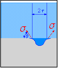
Fig. 4.49. Description of depression to explain the instability.

To analyze it, considered two control volumes bounded by the blue lines in Figure 4.49. The first control volume is made of a cylinder with a radius \(r\) and the second is the depression below it. The "extra" lines of the depression should be ignored, they are not part of the control volume. The horizontal forces around the control volume are canceling each other. At the top, the force is atmospheric pressure times the area. At the cylinder bottom, the force is \(\rho g h \times A\). This acts against the gravity force which make the cylinder to be in equilibrium with its surroundings if the pressure at bottom is indeed \(\rho g h\). For the depression, the force at the top is the same force at the bottom of the cylinder. At the bottom, the force is the integral around the depression. It can be approximated as a flat cylinder that has depth of \(r \pi / 4 \) (read the explanation in example 4.23). This value is exact if the shape is a perfect half sphere. In reality, the error is not significant. Additionally when the depression occurs, the liquid level is reduced a bit and the lighter liquid is filling the missing portion. Thus, the force at the bottom is \[F_{bottom} \sim \pi r^{2} \left[ \left( \frac{\pi r}{4} + h\right) \left(\rho_{L} - \rho_{G}\right) g + P_{atmos}\right] \] The net force is then \[F_{bottom} \sim \pi r^{2} \left(\frac{\pi r}{4} \right) \left( \rho_{L} - \rho_{G}\right) g \] The force that hold this column is the surface tenstion. As shown in fig. 4.49, the total force is then \[F_{\sigma} = 2\pi r \sigma cos \theta \] The forces balance on the depression is then \[2 \pi r \sigma cos \theta \sim \pi r^{2} \left(\frac{\pi r}{4}\right) \left( \rho_{L} - \rho_{G}\right) g \] The radius is obtained by \[r \sim \sqrt{\frac{2 \pi \sigma cos \theta}{\left( \rho_{L} - \rho_{G}\right) g}}\] The maximum surface tension is when the angle, \(\theta = \pi / 2\). At that case, the radius is \[r \sim \sqrt{\frac{2 \pi \sigma}{\left( \rho_{L} - \rho_{G}\right) g}}\]

Fig. 4.50. The cross section of the interface. The purple color represents the maximum heavy liquid raising area. The yellow color represents the maximum lighter liquid that "goes down."

The maximum possible radius of the depression depends on the geometry of the container. For the cylindrical geometry, the maximum depression radius is about half for the container radius (see Figure 4.50). This radius is limited because the lighter liquid has to enter at the same time into the heavier liquid zone. Since the "exchange'' volumes of these two process are the same, the specific radius is limited. Thus, it can be written that the minimum radius is \[r_{min tube} = 2\sqrt{\frac{2\pi\sigma}{g\left(\rho_{L} - \rho_{G}\right)}}\] The actual radius will be much larger. The heavier liquid can stay on top of the lighter liquid without being turned upside down when the radius is smaller than the equation 78. This analysis introduces a new dimensional number that will be discussed in a greater length in the Dimensionless chapter. In equation 78 the angle was assumed to be 90 degrees. However, this angle is never can be obtained. The actual value of this angle is about \(\pi/4\) to \(\pi/3\) and in only extreme cases the angle exceed this value (considering dynamics). In Figure 4.50, it was shown that the depression and the raised area are the same. The actual area of the depression is only a fraction of the interfacial cross section and is a function. For example,the depression is larger for square area. These two scenarios should be inserting into equation 4.168 by introducing experimental coefficient.

Example 4.33:

Estimate the minimum radius to insert liquid aluminum into represent tube at temperature of 600\([K]\). Assume that the surface tension is \(400[mN/m]\). The density of the aluminum is \(2400kg/m^3\).

Solution 4.33:

The depression radius is assume to be significantly smaller and thus equation (77) can be used. The density of air is negligible as can be seen from the temperature compare to the aluminum density.

\[ r \sim \sqrt{\dfrac{8\,\pi\,\overbrace{0.4}^{\sigma}}{ 2400\times 9.81}}
\]

The minimum radius is \(r \sim 0.02 [m]\) which demonstrates the assumption of \(h>>r\) was appropriate.

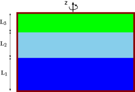
Fig. 4.51. Three liquids layers under rotation with various critical situations.

Open Question by April 15, 2010

The best solution of the following question will win 18 U.S. dollars and your name will be associated with the solution in this book.

Example 4.34:

A canister shown in Figure 4.51 has three layers of different fluids with different densities. Assume that the fluids do not mix. The canister is rotate with circular velocity, \(ω\). Describe the interface of the fluids consider all the limiting cases. Is there any difference if the fluids are compressible? Where is the maximum pressure points? For the case that the fluids are compressible, the canister top center is connected to another tank with equal pressure to the canister before the rotation (the connection point). What happen after the canister start to be rotated? Calculated the volume that will enter or leave, for known geometries of the fluids. Use the ideal gas model. You can assume that the process is isothermal. Is there any difference if the process is isentropic? If so, what is the difference?

Contributors and Attributions

• Dr. Genick Bar-Meir. Permission is granted to copy, distribute and/or modify this document under the terms of the GNU Free Documentation License, Version 1.2 or later or Potto license.