7.1: The First Law of Thermodynamics

This chapter focuses on the energy conservation which is the first law of thermodynamics . The fluid, as all phases and materials, obeys this law which creates strange and wonderful phenomena such as a shock and choked flow. Moreover, this law allows to solve problems, which were assumed in the previous chapters. For example, the relationship between height and flow rate was assumed previously, here it will be derived. Additionally a discussion on various energy approximation is presented. It was shown in Chapter 2 that the energy rate equation (??) for a system is

\[ \label{ene:eq:start}
\dot{Q} - \dot{W} = \dfrac{D\,E_U} {Dt} +
\dfrac{D\left(m\,U^2\right)} {Dt} + \dfrac{D\left(m\,g\,z\right)} {Dt}
\]

This equation can be rearranged to be

\[ \label{ene:eq:preRTT}
\dot{Q} - \dot{W} = \dfrac{D}{Dt} \,\left( E_U + m \, \dfrac{U^2}{2} + m \,g \, z \right)
\] Equation (2) is similar to equation (??) in which the right hand side has to be interpreted and the left hand side interpolated using the Reynold's Transport Theorem (RTT) . The right hand side is very complicated and only some of the effects will be discussed (It is only an introductory material). The energy transfer is carried (mostly ) by heat transfer to the system or the control volume. There are three modes of heat transfer, conduction, convection and radiation. In most problems, the radiation is minimal. Hence, the discussion here will be restricted to convection and conduction. Issues related to radiation are very complicated and considered advance material and hence will be left out. The issues of convection are mostly covered by the terms on the left hand side. The main heat transfer mode on the left hand side is conduction. Conduction for most simple cases is governed by Fourier's Law which is

\[ \label{ene:eq:fourier}
d\dot{q} = k_T \dfrac{dT}{dn} dA
\] Where \(d\dot{q}\) is heat transfer to an infinitesimal small area per time and \(k_T\) is the heat conduction coefficient. The heat derivative is normalized into area direction. The total heat transfer to the control volume is

\[ \label{ene:eq:tFourier}
\dot{Q} = \int_{A_{cv}} k \dfrac{dT}{dn} dA
\]

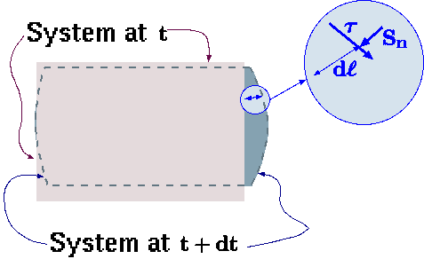
Fig. 7.1 The work on the control volume is done by two different mechanisms, \(S_n\) and \(\tau\).

The work done on the system is more complicated to express than the heat transfer. There are two kinds of works that the system does on the surroundings. The first kind work is by the friction or the shear stress and the second by normal force. As in the previous chapter, the surface forces are divided into two categories: one perpendicular to the surface and one with the surface direction. The work done by system on the surroundings (see Figure 7.1) is

\[ \label{ene:eq:dw}
dw = \overbrace{- \pmb{S} \, d\pmb{A}}^{d\pmb{F}} \cdot dll =
- \left( \pmb{S_n} + \boldsymbol{\tau} \right) \cdot \overbrace{d\pmb{ll} dA}^{dV}
\]

The change of the work for an infinitesimal time (excluding the shaft work) is

\[ \label{ene:eq:dwdt}
\dfrac{dw}{dt} = - \left( \pmb{S_n} + \boldsymbol{\tau} \right) \cdot \overbrace{\dfrac{d\pmb{ll}}{dt}}^{U} dA
= - \left( \pmb{S_n} + \boldsymbol{\tau} \right) \cdot \pmb{U}\, dA
\]
The total work for the system including the shaft work is

\[ \label{mom:eq:tW}
\dot{W} = -\int_{A{c.v.}} \left( \pmb{S_n} + \boldsymbol{\tau} \right)\,\pmb{U} \, dA - W_{shaft}
\] The energy equation (2) for system is

\[ \label{eye:eq:sysE}
\displaystyle \int_{A_{sys}} k_T \dfrac{dT}{dn} dA +
\displaystyle \int_{A_{sys}} \left( \pmb{S_n} + \boldsymbol{\tau} \right) \, dV \\
+ \dot{W}_{shaft} =
\dfrac{D}{Dt} \displaystyle \int_{V_{sys}} \rho\, \left( E_U + m \, \dfrac{U^2}{2} + g \, z \right) dV
\] Equation (8) does not apply any restrictions on the system. The system can contain solid parts as well several different kinds of fluids. Now Reynolds Transport Theorem can be used to transformed the left hand side of equation (8) and thus yields

Energy Equation

\[ \label{eye:eq:cvE}
\begin{array}[t]{l}
\displaystyle \int_{A_{cv}} k_T \dfrac{dT}{dn} dA + \displaystyle \int_{A_{cv}} \left( \pmb{S_n} +
\boldsymbol{\tau} \right) \, dA + \dot{W}_{shaft} = \\
\dfrac{d}{dt} \displaystyle \int_{V_{cv}} \rho\, \left( E_u + m \, \dfrac{U^2}{2} + g \, z \right) dV \\
\displaystyle
+ \displaystyle \int_{A_{cv}} \left( E_u + m \, \dfrac{U^2}{2} + g \, z \right)\,\rho\, U_{rn} dA
\end{array}
\]

From now on the notation of the control volume and system will be dropped since all equations deals with the control volume. In the last term in equation (9) the velocity appears twice. Note that \(U\) is the velocity in the frame of reference while \(U_{rn}\) is the velocity relative to the boundary. As it was discussed in the previous chapter the normal stress component is replaced by the pressure (see equation (??) for more details). The work rate (excluding the shaft work) is

\[ \label{ene:eq:workRate0}
\dot{W} \cong \overbrace{\int_S P \hat{n} \cdot \pmb{U} dA}^{\text{ flow $\,\,$ work} } -
\int_S \boldsymbol{\tau} \cdot \pmb{U} \,\hat{n}\, dA
\]

The first term on the right hand side is referred to in the literature as the flow work and is

\[ \label{ene:eq:flowWork1}
\int_S P \hat{n} \cdot \pmb{U} dA = \int_S P \overbrace{\left(U - U_b\right)\hat{n} }^{U_{rn}} dA +
\int_S P\, U_{bn} dA
\] Equation (11) can be further manipulated to become

\[ \label{ene:eq:flowWorkF}
\int_S P \hat{n} \cdot \pmb{U} dA = \overbrace{\int_S \dfrac{P}{\rho} \, \rho\, U_{rn}\, dA}
^{\text{ work due to the flow}} +
\overbrace{\int_S P U_{bn} dA}^{\text{ work due to boundaries movement}}
\] The second term is referred to as the shear work and is defined as

\[ \label{ene:eq:shearW}
\dot{W}_{shear} = -\int_S \boldsymbol{\tau}\cdot \pmb{U} dA
\] Substituting all these terms into the governing equation yields

\[ \label{ene:eq:governingE1}
\dot{Q} - \dot{W}_{shear} - \dot{W}_{shaft} = \dfrac{d}{dt} \displaystyle \int_V
\left( E_u + \dfrac{U^2}{2\dfrac{}{}} + g\,z\right) dV + \\
\displaystyle \int_S \left( E_u + \dfrac{P}{\rho} + \dfrac{U^2} {2\dfrac{}{}} + g\,z \right) U_{rn}\, \rho \,dA +
\displaystyle \int_S P U_{rn} dA
\] The new term \(P/\rho\) combined with the internal energy, \(E_u\) is referred to as the enthalpy, \(h\), which was discussed on page ??. With these definitions equation (14) transformed

Simplified Energy Equation

\[ \label{ene:eq:governingE}
\begin{array}{l}
\dot{Q} - \dot{W}_{shear} + \dot{W}_{shaft} = \dfrac{d}{dt} \displaystyle \int_V \left( E_u + \dfrac{U^2}{2}
+ g\,z\right) \,\rho\,dV + \\
\displaystyle \int_S \left( h + \dfrac{U^2} {2} + g\,z \right) U_{rn}\, \rho \,dA +
\displaystyle \int_S P U_{bn} dA
\end{array}
\]

Equation (15) describes the energy conservation for the control volume in stationary coordinates. Also note that the shear work inside the the control volume considered as shaft work. The example of flow from a tank or container is presented to demonstrate how to treat some of terms in equation (15).

Flow Out From A Container

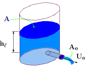
Fig. 7.2 Discharge from a Large Container with a small diameter.

In the previous chapters of this book, the flow rate out of a tank or container was assumed to be a linear function of the height. The flow out is related to the height but in a more complicate function and is the focus of this discussion. The energy equation with mass conservation will be utilized for this analysis. In this analysis several assumptions are made which includes the following: constant density, the gas density is very small compared to liquid density, and exit area is relatively small, so the velocity can be assumed uniform (not a function of the opening surface tension effects are negligible and the liquid surface is straight . Additionally, the temperature is assumed to constant. The control volume is chosen so that all the liquid is included up to exit of the pipe. The conservation of the mass is

\[ \label{ene:eq:Tmass}
\dfrac{d}{dt} \int_V \cancel{\rho}\,dV + \int_A \cancel{\rho} \, U_{rn} \, dA =0
\]

which also can be written (because \(\dfrac{d\rho}{dt} = 0\)) as

\[ \label{ene:eq:TmassB}
\int_A U_{bn} \, dA + \int_A U_{rn} dA = 0
\] Equation (17) provides the relationship between boundary velocity to the exit velocity as

\[ \label{ene:eq:TmF}
A\,U_b = A_e\,U_e
\] Note that the boundary velocity is not the averaged velocity but the actual velocity. The averaged velocity in \(z\) direction is same as the boundary velocity

\[ \label{ene:eq:TUzUb}
U_b = U_z = \dfrac{dh}{dt} = \dfrac{A_e}{A}\,U_e
\] The \(x\) component of the averaged velocity is a function of the geometry and was calculated in Example to be larger than

\[ \label{ene:eq:TbarUx}
\overline{U_x} \precapprox \dfrac{2\,r}{h} \dfrac{A_e}{A} U_e \Longrightarrow
\overline{U_x} \cong \dfrac{2\,r}{h}\,U_b = \dfrac{2\,r}{h}\,\dfrac{dh}{dt}
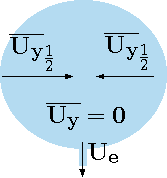
\] In this analysis, for simplicity, this quantity will be used. The averaged velocity in the \(y\) direction is zero because the flow is symmetrical . However, the change of the kinetic energy due to the change in the velocity field isn't zero. The kinetic energy of the tank or container is based on the half part as shown in Figure 7.3. Similar estimate that was done for \(x\) direction can be done to every side of the opening if they are not symmetrical. Since in this case the geometry is assumed to be symmetrical one side is sufficient as

\[ \label{ene:eq:TUzave}
\overline{U_y} \cong \dfrac{ (\pi - 2) r}{8\,h} \dfrac{dh}{dt}
\]

Fig. 7.3 How to compensate and estimate the kinetic energy when averaged Velocity is zero.

The energy balance can be expressed by equation (15) which is applicable to this case. The temperature is constant. In this light, the following approximation can be written

\[ \label{ene:eq:Tc}
\dot{Q} = \dfrac{E_u}{dt} = h_{in} - h_{out} = 0
\]

The boundary shear work is zero because the velocity at tank boundary or walls is zero. Furthermore, the shear stresses at the exit are normal to the flow direction hence the shear work is vanished. At the free surface the velocity has only normal component and thus shear work vanishes there as well. Additionally, the internal shear work is assumed negligible.

\[ \label{ene:eq:noWs}
\dot{W}_{shear} = \dot{W}_{shaft} = 0
\] Now the energy equation deals with no "external'' effects. Note that the (exit) velocity on the upper surface is zero \(U_{rn}=0\). Combining all these information results in

\[ \label{ene:eq:Tenergy}
\overbrace{\dfrac{d}{dt} \int_V \left( \dfrac{U^2}{2} + g\,z\right) \rho\, dV}^
{\text{ internal energy change}} +
\overbrace{\overbrace{\int_A \left( \dfrac{P_e}{\rho} + \dfrac

ParseError: EOF expected (click for details)

Callstack:
    at (Bookshelves/Civil_Engineering/Book:_Fluid_Mechanics_(Bar-Meir)/07:_Energy_Conservation/7.1:_The_First_Law_of_Thermodynamics), /content/body/div[3]/p[15]/span, line 1, column 4

-
\overbrace{\int_A P_a\, U_b\,dA}^
{\text{ upper surface work }} } ^
{\text{energy flow out }} = 0
\] Where \(U_b\) is the upper boundary velocity, \(P_a\) is the external pressure and \(P_e\) is the exit pressure . The pressure terms in equation (24) are

\[ \label{ene:eq:Tp1}
\int_A \dfrac{P_e}{\rho}\, U_e\, \rho dA - \int_A P_a\, U_b\, dA =
P_e\, \int_A U_e\, dA - P_a\,\int_A U_b\, dA
\] It can be noticed that \(P_a = P_e\) hence

\[ \label{ene:eq:Tp1a}
P_a \overbrace{\left( \int_A U_e\, dA - \int_A U_b\, dA \right)}^{=0} = 0
\] The governing equation (24) is reduced to

\[ \label{ene:eq:TenergyF1}
{\dfrac{d}{dt} \int_V \left( \dfrac{U^2}{2} + g\,z\right) \rho\, dV} -
\int_A \left( \dfrac

ParseError: EOF expected (click for details)

Callstack:
    at (Bookshelves/Civil_Engineering/Book:_Fluid_Mechanics_(Bar-Meir)/07:_Energy_Conservation/7.1:_The_First_Law_of_Thermodynamics), /content/body/div[3]/p[18]/span[1], line 1, column 4

^2\, V = \rho \left( \dfrac{1}{V}\int_V U dV \right)^2 \,V = \rho \left( \int_V U dV \right)^2 \] The general correction factor is the ratio of the above value to the actual kinetic energy as \[ \label{ene:eq:CFene} C_F = \dfrac{\left( \displaystyle\int_V \rho\, U\, dV \right)^2 } { \displaystyle \int_V \rho\,U^2\, dV } eq \dfrac{\cancel{\rho}\, \left( U_{ave} \right)^2\,V } { \displaystyle \int_V \cancel{\rho}\,U^2\, dV } \] Here, \(C_F\) is the correction coefficient. Note, the inequality sign because the density distribution for compressible fluid. The correction factor for a constant density fluid is \[ \label{ene:eq:CFeneNC} C_F = \dfrac{\left( \displaystyle\int_V \rho\, U\, dV \right)^2 } { \displaystyle \int_V \rho\,U^2\, dV } = \dfrac{\left(\cancel{\rho}\, \displaystyle\int_V U\, dV \right)^2 } { \cancel{\rho}\,\displaystyle \int_V U^2\, dV } = \dfrac{ {U_{ave}}^2\,V } { \displaystyle \int_V U^2\, dV } \] This integral can be evaluated for any given velocity profile. A large family of velocity profiles is laminar or parabolic (for one directional flow) . For a pipe geometry, the velocity is \[ \label{ene:eq:parabolic} U \left(\dfrac{r}{R}\right) = {U}\,(\bar{r}) = U_{max} \left( 1-\bar{r}^2 \right) = 2\,U_{ave} \left( 1-\bar{r}^2 \right) \] It can be noticed that the velocity is presented as a function of the reduced The relationship between \(U_{max}\) to the averaged velocity, \(U_{ave}\) is obtained by using equation (32) which yields \(1/2\). Substituting equation (36) into equation (35) results \[ \label{ene:eq:eneAve} \dfrac{ {U_{ave}}^2\,V }{ \displaystyle \int_V U^2\, dV } = \dfrac{ {U_{ave}}^2\,V } {\displaystyle \int_V \left( 2\,U_{ave} \left( 1-\bar{r}^2 \right) \right)^2\, dV } = \dfrac{ {U_{ave}}^2\,V } {\dfrac{4\,{U_{ave}}^2\,\pi\,L\,R^2}{3} } = \dfrac{3}{4} \] The correction factor for many other velocity profiles and other geometries can be smaller or larger than this value. For circular shape, a good guess number is about 1.1. In this case, for simplicity reason, it is assumed that the averaged velocity indeed represent the energy in the tank or container. Calculations according to this point can improve the accurately based on the above discussion. \cBox{ The difference between the "averaged momentum'' velocity and the "averaged kinetic'' velocity is also due to the fact that energy is added for different directions while in the momentum case, different directions cancel each other out.} The unsteady state term then obtains the form \[ \begin{array}{rl} \label{ene:eq:unstadyT} \dfrac{d}{dt} \displaystyle \int_V \rho\,\left( \dfrac{U^2}{2} + g\,y\right) \, dV & \cong \rho\, \dfrac{d}{dt} \left( \left[ \dfrac

ParseError: invalid DekiScript (click for details)

Callstack:
    at (Bookshelves/Civil_Engineering/Book:_Fluid_Mechanics_(Bar-Meir)/07:_Energy_Conservation/7.1:_The_First_Law_of_Thermodynamics), /content/body/div[3]/p[18]/span[2], line 1, column 1

^2 \cong {\overline{U_x}}^2 + {\overline{U_y}}^2 + {\overline{U_z}}^2
\]

\[ \label{ene:eq:TuaveIntermite}
{\overline{U}}^2 \cong \left(\dfrac{\left(\pi - 2\right)r}{8\,h} \dfrac{dh}{dt}\right)^2 +
\left(\dfrac{\left(\pi - 1\right)r}{4\,h} \dfrac{dh}{dt}\right)^2 +
\left(\dfrac{dh}{dt}\right)^2
\]

\[ \label{ene:eq:TuaveF}
{\overline{U}} \cong \dfrac{dh}{dt} \,\,
\overbrace{\sqrt{\left(\dfrac{\left(\pi - 2\right)r}{8\,h} \right)^2 +
\left(\dfrac{\left(\pi - 1\right)r}{4\,h} \right)^2 + 1^2}}^{f(G)}
\] It can be noticed that \(f(G)\) is a weak function of the height inverse. Analytical solution of the governing equation is possible including this effect of the height. However, the mathematical complication are enormous and this effect is assumed negligible and the function to be constant. The last term is

\[ \label{ene:eq:TEnergyOut}
\int_A \dfrac

ParseError: EOF expected (click for details)

Callstack:
    at (Bookshelves/Civil_Engineering/Book:_Fluid_Mechanics_(Bar-Meir)/07:_Energy_Conservation/7.1:_The_First_Law_of_Thermodynamics), /content/body/div[3]/p[21]/span, line 1, column 4

\\
- \dfrac{1}{2}\left( \dfrac{dh}{dt} \right)^2 \left( \dfrac{A}{A_e}\right)^2\, {U_e \,A_e} = 0
\] Equation (47) can be rearranged and simplified and combined with mass conservation

Advance Material

Dividing equation (46) by \(U_e\)\(A_e\) and utilizing equation (40)

\[ \label{ene:eq:TenergyFb}
\dfrac{d}{dt} \left[ \dfrac

ParseError: invalid DekiScript (click for details)

Callstack:
    at (Bookshelves/Civil_Engineering/Book:_Fluid_Mechanics_(Bar-Meir)/07:_Energy_Conservation/7.1:_The_First_Law_of_Thermodynamics), /content/body/div[3]/p[24]/span, line 1, column 1

^{A\,\dfrac{A_e}{A}{U_e}}
- \dfrac{1}{2}\left( \dfrac{dh}{dt} \right)^2 \left( \dfrac{A}{A_e}\right)^2\, \cancel{U_e \,A_e} = 0
\]

Notice that \(\overline{U} = U_b\,f(G)\) and thus

\[ \label{ene:eq:TenergyFba}
\overbrace{\overline{U}}^{f(G)\,U_b}
\dfrac{d \overline{U}}{dt} \dfrac{h\, A}{U_e \,A_e} + \dfrac{g}{2} \dfrac{dh}{dt} \,
\dfrac{h\, A}{U_e \,A_e} + \left[ \dfrac{{\overline{U}}^2}{2} + \dfrac{g\,h}{2} \right] \\ - \dfrac{1}{2} \left( \dfrac{dh}{dt} \right)^2 \left( \dfrac{A}{A_e}\right)^2 = 0 \] Further rearranging to eliminate the "flow rate'' transforms to \[ \label{ene:eq:TenergyFc} f(G)\, h\,\dfrac{d \overline{U}}{dt} \cancelto{1}{\left(\dfrac{{U_b}\,A}{U_e \,A_e}\right)} + \dfrac{g\,h}{2} \, \cancelto{1}{\dfrac{\dfrac{dh}{dt}\, A}{U_e \,A_e}} + \\
\left[ \dfrac{f(G)^2}{2} \left(\dfrac{dh}{dt}\right)^2 + \dfrac{g\,h}{2} \right]
- \dfrac{1}{2} \left( \dfrac{dh}{dt} \right)^2 \left( \dfrac{A}{A_e}\right)^2 = 0
\]

\[ \label{ene:eq:TenergyFd}
f(G)^2\, h\,\dfrac{d^2 h }{dt^2}
+ \dfrac{g\,h}{2} + \left[ \dfrac{f(G)^2}{2} \left(\dfrac{dh}{dt}\right)^2 + \dfrac{g\,h}{2} \right]
- \dfrac{1}{2} \left( \dfrac{dh}{dt} \right)^2 \left( \dfrac{A}{A_e}\right)^2 = 0
\]

End Advance Material

Combining the \(gh\) terms into one yields

\[ \label{ene:eq:TenergyFe}
f(G)^2\, h\,\dfrac{d^2 h }{dt^2}
+ g\,h + \dfrac{1}{2} \left(\dfrac{dh}{dt}\right)^2\left[ {f(G)^2}
- \left( \dfrac{A}{A_e}\right)^2 \right]
= 0
\]

Defining a new tank emptying parameter, \(T_e\), as

\[ \label{ene:eq:EmptyParamer}
T_e = \left( \dfrac{A}{f(G)\, A_e}\right)^2
\] This parameter represents the characteristics of the tank which controls the emptying process. Dividing equation (52) by \(f(G)^2\) and using this parameter, equation (52) after minor rearrangement transformed to

\[ \label{ene:eq:TenergyFeGaa}
h \left( \,\dfrac{d^2 h }{dt^2} + \dfrac{g\,{A_e}^2}{T_e\,A^2}\right) +
\dfrac{1}{2} \left(\dfrac{dh}{dt}\right)^2\left[ 1 - T_e \right]
= 0
\] The solution can either of these equations

\[ \label{ene:eq:Tsol1T}
-\int \dfrac{dh}
{\sqrt{\dfrac{\left( k_1\,T_e-2\,k_1\right)
\,{e}^{\ln \left( h\right) \,Te}+2\,g\,{h}^{2}}{h\,
\left( {Te}-2\right) \,f(G) } }
}
= t + k_2
\] or

\[ \label{ene:eq:Tsol2T}
\int \dfrac{dh}
{\sqrt{\dfrac{\left( k_1\,T_e-2\,k_1\right)
\,{e}^{\ln \left( h\right) \,Te}+2\,g\,{h}^{2}}{h\,
\left( {Te}-2\right) \,f(G) } }
}
= t + k_2
\] The solution with the positive solution has no physical meaning because the height cannot increase with time. Thus define function of the height as

\[ \label{ene:eq:Th}
f(h) =
-\int \dfrac{dh}
{\sqrt{\dfrac{\left( k_1\,T_e-2\,k_1\right)
\,{e}^{\ln \left( h\right) \,Te}+2\,g\,{h}^{2}}{h\,
\left( {Te}-2\right) \,f(G) } }
}
\]
The initial condition for this case are: one the height initial is

\[ \label{ene:eq:Tinih0}
h(0) = h_0
\] The initial boundary velocity is

\[ \label{ene:eq:Tinih1}
\dfrac{dh}{dt} = 0
\] This condition pose a physical limitation which will be ignored. The first condition yields

\[ \label{ene:eq:TiniP0}
k_2 = - f(h_0)
\]

The second condition provides

\[ \label{ene:eq:TiniP1}
\dfrac{dh}{dt} = 0 =
\sqrt{\dfrac{\left( k_1\,T_e-2\,k_1\right)
\,{e}^{\ln \left( h_0\right) \,Te}+2\,g\,{h_0}^{2}}{h_0\,
\left( {Te}-2\right) \,f(G) } }
\]

The complication of the above solution suggest a simplification in which

\[ \label{ene:eq:simplificaitonCondition}
\dfrac{d^2 h }{dt^2} << \dfrac{g\,{A_e}^2}{T_e\,A^2}
\] which reduces equation (54) into

\[ \label{ene:eq:TenergyFeG}
h \left( \dfrac{g\,{A_e}^2}{T_e\,A^2}\right) +
\dfrac{1}{2} \left(\dfrac{dh}{dt}\right)^2\left[ 1 - T_e \right]
= 0
\] While equation (63) is still non linear equation, the non linear element can be removed by taking negative branch (height reduction) of the equation as

\[ \label{ene:eq:dhdt2}
\left( \dfrac{dh}{dt} \right)^2 = \dfrac{ 2\,g\,h}{ -1 + \left( \dfrac{A}{A_e}\right)^2 }
\] It can be noticed that \(T_e\) "disappeared'' from the equation. And taking the "positive'' branch

\[ \label{ene:eq:dhdt}
\dfrac{dh}{dt} = \dfrac{ \sqrt{2\,g\,h} } { \sqrt{1 - \left( \dfrac{A}{A_e}\right)^2 } }
\] The nature of first order Ordinary Differential Equation that they allow only one initial condition. This initial condition is the initial height of the liquid. The initial velocity field was eliminated by the approximation (remove the acceleration term). Thus it is assumed that the initial velocity is not relevant at the core of the process at hand. It is correct only for large ratio of \(h/r\) and the error became very substantial for small value of \(h/r\). Equation (65) integrated to yield

\[ \label{ene:eq:hInt}
\left({ 1 - \left( \dfrac{A}{A_e}\right)^2 }\right) \int_{h_0}^h \dfrac{dh}{\sqrt{2\,g\,h}} =
\int_0^t dt
\] The initial condition has been inserted into the integral which its solution is

\[ \label{ene:eq:tankS}
\left({ 1 - \left( \dfrac{A}{A_e}\right)^2 }\right)\, \dfrac{h-h_0}{\sqrt{2\,g\,h}} = t
\]

\[ \label{ene:eq:tAppx}
U_e = \dfrac{dh}{dt} \dfrac{A}{A_e} =
\dfrac{ \sqrt{2\,g\,h} } { \sqrt{1 - \left( \dfrac{A}{A_e}\right)^2 }} \dfrac{A}{A_e}
= \dfrac{ \sqrt{2\,g\,h} } {\sqrt{ 1 - \left( \dfrac{A_e}{A}\right)^2 }}
\] If the area ratio \(A_e/A << 1\) then

\[ \label{ene:eq:torricelli}
U \cong \sqrt{2\,g\,h}
\] Equation (69) is referred in the literature as Torricelli's equation This analysis has several drawbacks which limits the accuracy of the calculations. Yet, this analysis demonstrates the usefulness of the integral analysis to provide a reasonable solution. This analysis can be improved by experimental investigating the phenomenon. The experimental coefficient can be added to account for the dissipation and other effects such

\[ \label{ene:eq:ExpCoefficient}
\dfrac{dh}{dt} \cong C\,\sqrt{2\,g\,h}
\] The loss coefficient can be expressed as

\[ \label{ene:eq:lossC}
C = K f\left( \dfrac{U^2}{2} \right)
\] A few loss coefficients for different configuration is given following Figure 7.4.

Figure 7.4 ypical resistance for selected outlet configuration. The sharp cover on the left with K=1, K=0.5 and 0.04 repsectivly on the right.

Contributors

• Dr. Genick Bar-Meir. Permission is granted to copy, distribute and/or modify this document under the terms of the GNU Free Documentation License, Version 1.2 or later or Potto license.