10.2.3: The Connection Between the Stream Function and the Potential Function
- Page ID
- 779
\( \newcommand{\vecs}[1]{\overset { \scriptstyle \rightharpoonup} {\mathbf{#1}} } \)
\( \newcommand{\vecd}[1]{\overset{-\!-\!\rightharpoonup}{\vphantom{a}\smash {#1}}} \)
\( \newcommand{\id}{\mathrm{id}}\) \( \newcommand{\Span}{\mathrm{span}}\)
( \newcommand{\kernel}{\mathrm{null}\,}\) \( \newcommand{\range}{\mathrm{range}\,}\)
\( \newcommand{\RealPart}{\mathrm{Re}}\) \( \newcommand{\ImaginaryPart}{\mathrm{Im}}\)
\( \newcommand{\Argument}{\mathrm{Arg}}\) \( \newcommand{\norm}[1]{\| #1 \|}\)
\( \newcommand{\inner}[2]{\langle #1, #2 \rangle}\)
\( \newcommand{\Span}{\mathrm{span}}\)
\( \newcommand{\id}{\mathrm{id}}\)
\( \newcommand{\Span}{\mathrm{span}}\)
\( \newcommand{\kernel}{\mathrm{null}\,}\)
\( \newcommand{\range}{\mathrm{range}\,}\)
\( \newcommand{\RealPart}{\mathrm{Re}}\)
\( \newcommand{\ImaginaryPart}{\mathrm{Im}}\)
\( \newcommand{\Argument}{\mathrm{Arg}}\)
\( \newcommand{\norm}[1]{\| #1 \|}\)
\( \newcommand{\inner}[2]{\langle #1, #2 \rangle}\)
\( \newcommand{\Span}{\mathrm{span}}\) \( \newcommand{\AA}{\unicode[.8,0]{x212B}}\)
\( \newcommand{\vectorA}[1]{\vec{#1}} % arrow\)
\( \newcommand{\vectorAt}[1]{\vec{\text{#1}}} % arrow\)
\( \newcommand{\vectorB}[1]{\overset { \scriptstyle \rightharpoonup} {\mathbf{#1}} } \)
\( \newcommand{\vectorC}[1]{\textbf{#1}} \)
\( \newcommand{\vectorD}[1]{\overrightarrow{#1}} \)
\( \newcommand{\vectorDt}[1]{\overrightarrow{\text{#1}}} \)
\( \newcommand{\vectE}[1]{\overset{-\!-\!\rightharpoonup}{\vphantom{a}\smash{\mathbf {#1}}}} \)
\( \newcommand{\vecs}[1]{\overset { \scriptstyle \rightharpoonup} {\mathbf{#1}} } \)
\( \newcommand{\vecd}[1]{\overset{-\!-\!\rightharpoonup}{\vphantom{a}\smash {#1}}} \)
\(\newcommand{\avec}{\mathbf a}\) \(\newcommand{\bvec}{\mathbf b}\) \(\newcommand{\cvec}{\mathbf c}\) \(\newcommand{\dvec}{\mathbf d}\) \(\newcommand{\dtil}{\widetilde{\mathbf d}}\) \(\newcommand{\evec}{\mathbf e}\) \(\newcommand{\fvec}{\mathbf f}\) \(\newcommand{\nvec}{\mathbf n}\) \(\newcommand{\pvec}{\mathbf p}\) \(\newcommand{\qvec}{\mathbf q}\) \(\newcommand{\svec}{\mathbf s}\) \(\newcommand{\tvec}{\mathbf t}\) \(\newcommand{\uvec}{\mathbf u}\) \(\newcommand{\vvec}{\mathbf v}\) \(\newcommand{\wvec}{\mathbf w}\) \(\newcommand{\xvec}{\mathbf x}\) \(\newcommand{\yvec}{\mathbf y}\) \(\newcommand{\zvec}{\mathbf z}\) \(\newcommand{\rvec}{\mathbf r}\) \(\newcommand{\mvec}{\mathbf m}\) \(\newcommand{\zerovec}{\mathbf 0}\) \(\newcommand{\onevec}{\mathbf 1}\) \(\newcommand{\real}{\mathbb R}\) \(\newcommand{\twovec}[2]{\left[\begin{array}{r}#1 \\ #2 \end{array}\right]}\) \(\newcommand{\ctwovec}[2]{\left[\begin{array}{c}#1 \\ #2 \end{array}\right]}\) \(\newcommand{\threevec}[3]{\left[\begin{array}{r}#1 \\ #2 \\ #3 \end{array}\right]}\) \(\newcommand{\cthreevec}[3]{\left[\begin{array}{c}#1 \\ #2 \\ #3 \end{array}\right]}\) \(\newcommand{\fourvec}[4]{\left[\begin{array}{r}#1 \\ #2 \\ #3 \\ #4 \end{array}\right]}\) \(\newcommand{\cfourvec}[4]{\left[\begin{array}{c}#1 \\ #2 \\ #3 \\ #4 \end{array}\right]}\) \(\newcommand{\fivevec}[5]{\left[\begin{array}{r}#1 \\ #2 \\ #3 \\ #4 \\ #5 \\ \end{array}\right]}\) \(\newcommand{\cfivevec}[5]{\left[\begin{array}{c}#1 \\ #2 \\ #3 \\ #4 \\ #5 \\ \end{array}\right]}\) \(\newcommand{\mattwo}[4]{\left[\begin{array}{rr}#1 \amp #2 \\ #3 \amp #4 \\ \end{array}\right]}\) \(\newcommand{\laspan}[1]{\text{Span}\{#1\}}\) \(\newcommand{\bcal}{\cal B}\) \(\newcommand{\ccal}{\cal C}\) \(\newcommand{\scal}{\cal S}\) \(\newcommand{\wcal}{\cal W}\) \(\newcommand{\ecal}{\cal E}\) \(\newcommand{\coords}[2]{\left\{#1\right\}_{#2}}\) \(\newcommand{\gray}[1]{\color{gray}{#1}}\) \(\newcommand{\lgray}[1]{\color{lightgray}{#1}}\) \(\newcommand{\rank}{\operatorname{rank}}\) \(\newcommand{\row}{\text{Row}}\) \(\newcommand{\col}{\text{Col}}\) \(\renewcommand{\row}{\text{Row}}\) \(\newcommand{\nul}{\text{Nul}}\) \(\newcommand{\var}{\text{Var}}\) \(\newcommand{\corr}{\text{corr}}\) \(\newcommand{\len}[1]{\left|#1\right|}\) \(\newcommand{\bbar}{\overline{\bvec}}\) \(\newcommand{\bhat}{\widehat{\bvec}}\) \(\newcommand{\bperp}{\bvec^\perp}\) \(\newcommand{\xhat}{\widehat{\xvec}}\) \(\newcommand{\vhat}{\widehat{\vvec}}\) \(\newcommand{\uhat}{\widehat{\uvec}}\) \(\newcommand{\what}{\widehat{\wvec}}\) \(\newcommand{\Sighat}{\widehat{\Sigma}}\) \(\newcommand{\lt}{<}\) \(\newcommand{\gt}{>}\) \(\newcommand{\amp}{&}\) \(\definecolor{fillinmathshade}{gray}{0.9}\)For this discussion, the situation of two dimensional incompressible is assumed. It was shown that
\[
\label{if:eq:UxpotentianlSteam}
\pmb{U}_x = \dfrac{\partial \phi}{\partial x}
= \dfrac{\partial \psi}{\partial y}
\]
and
\[
\label{if:eq:UypotentianlSteam}
\pmb{U}_y = \dfrac{\partial \phi}{\partial y}
= - \dfrac{\partial \psi}{\partial x}
\]
These equations (70) and (71) are referred to Definition of the potential function is based on the gradient operator as \(\pmb{U} = \boldsymbol{\nabla}\phi\) thus derivative in arbitrary direction can be written as
\[
\label{if:eq:arbitraryPotential}
\dfrac{d\phi}{ds} = \boldsymbol{\nabla}\phi \boldsymbol{\cdot} \widehat{s} =
\pmb{U} \boldsymbol{\cdot} \widehat{s}
\]
\[
\label{if:eq:velocitystreamPotential}
{U} = \dfrac{d\phi}{ds}
\]
If the derivative of the stream function is chosen in the direction of the flow then as in was shown in equation (58). It summarized as
\[
\label{if:eq:streamFpotentialFDerivative}
\dfrac{d\phi}{ds} = \dfrac{d\psi}{dn}
\]
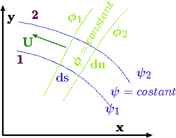
Fig. 10.3 Constant Stream lines and Constant Potential lines.
There are several conclusions that can be drawn from the derivations above. The conclusion from equation (74) that the stream line are orthogonal to potential lines. Since the streamline represent constant value of stream function it follows that the potential lines are constant as well. The line of constant value of the potential are referred as potential lines.
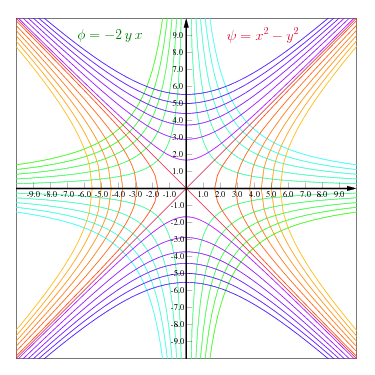
Fig. 10.4 Stream lines and potential lines are drawn as drawn for two dimensional flow. The green to green–turquoise color are the potential lines. Note that opposing quadrants (first and third quadrants) have the same colors. The constant is larger as the color approaches the turquoise color. Note there is no constant equal to zero while for the stream lines the constant can be zero. The stream line are described by the orange to blue lines. The orange lines describe positive constant while the purple lines to blue describe negative constants. The crimson line are for zero constants. This Figure was part of a project by Eliezer Bar-Meir to learn GLE graphic programing language.
Figure 10.4 describes almost a standard case of stream lines and potential lines.
Example 10.3
A two dimensional stream function is given as \(\psi= x^4 - y^2\). Calculate the expression for the potential function \(\phi\) (constant value) and sketch the streamlines lines (of constant value).
Solution 10.3
Utilizing the differential equation (70) and (??) to
\[
\label{streamTOpotential:derivativeY}
\dfrac{\partial \phi}{\partial x} =
\dfrac{\partial \psi}{\partial y} = - 2\, y
\]
\[
\label{streamTOpotential:integralX}
\phi = - 2\,x\,y + f(y)
\]
where \(f(y)\) is arbitrary function of \(y\). Utilizing the other relationship (??) leads
\[
\label{streamTOpotential:eq:derivativeX}
\dfrac{\partial \phi}{\partial y} = - 2\, x + \dfrac{d\,f(y) }{dy} =
- \dfrac{\partial \psi}{\partial x} = - 4\,x^3
\]
Therefore
\[
\label{streamTOpotential:eq:potentialODE}
\dfrac{d\,f(y) }{dy} = 2\,x - 4\, x^3
\]
After the integration the function \(\phi\) is
\[
\label{streamTOpotential:phiIntegration}
\phi = \left( 2\,x - 4\, x^3 \right)\, y + c
\]
The results are shown in Figure
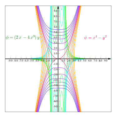
Fig. 10.5 Stream lines and potential lines for Example .
Template:HideTOC
Contributors and Attributions
Dr. Genick Bar-Meir. Permission is granted to copy, distribute and/or modify this document under the terms of the GNU Free Documentation License, Version 1.2 or later or Potto license.