5.1: Initiation of Motion of Particles
- Page ID
- 29206
\( \newcommand{\vecs}[1]{\overset { \scriptstyle \rightharpoonup} {\mathbf{#1}} } \)
\( \newcommand{\vecd}[1]{\overset{-\!-\!\rightharpoonup}{\vphantom{a}\smash {#1}}} \)
\( \newcommand{\id}{\mathrm{id}}\) \( \newcommand{\Span}{\mathrm{span}}\)
( \newcommand{\kernel}{\mathrm{null}\,}\) \( \newcommand{\range}{\mathrm{range}\,}\)
\( \newcommand{\RealPart}{\mathrm{Re}}\) \( \newcommand{\ImaginaryPart}{\mathrm{Im}}\)
\( \newcommand{\Argument}{\mathrm{Arg}}\) \( \newcommand{\norm}[1]{\| #1 \|}\)
\( \newcommand{\inner}[2]{\langle #1, #2 \rangle}\)
\( \newcommand{\Span}{\mathrm{span}}\)
\( \newcommand{\id}{\mathrm{id}}\)
\( \newcommand{\Span}{\mathrm{span}}\)
\( \newcommand{\kernel}{\mathrm{null}\,}\)
\( \newcommand{\range}{\mathrm{range}\,}\)
\( \newcommand{\RealPart}{\mathrm{Re}}\)
\( \newcommand{\ImaginaryPart}{\mathrm{Im}}\)
\( \newcommand{\Argument}{\mathrm{Arg}}\)
\( \newcommand{\norm}[1]{\| #1 \|}\)
\( \newcommand{\inner}[2]{\langle #1, #2 \rangle}\)
\( \newcommand{\Span}{\mathrm{span}}\) \( \newcommand{\AA}{\unicode[.8,0]{x212B}}\)
\( \newcommand{\vectorA}[1]{\vec{#1}} % arrow\)
\( \newcommand{\vectorAt}[1]{\vec{\text{#1}}} % arrow\)
\( \newcommand{\vectorB}[1]{\overset { \scriptstyle \rightharpoonup} {\mathbf{#1}} } \)
\( \newcommand{\vectorC}[1]{\textbf{#1}} \)
\( \newcommand{\vectorD}[1]{\overrightarrow{#1}} \)
\( \newcommand{\vectorDt}[1]{\overrightarrow{\text{#1}}} \)
\( \newcommand{\vectE}[1]{\overset{-\!-\!\rightharpoonup}{\vphantom{a}\smash{\mathbf {#1}}}} \)
\( \newcommand{\vecs}[1]{\overset { \scriptstyle \rightharpoonup} {\mathbf{#1}} } \)
\( \newcommand{\vecd}[1]{\overset{-\!-\!\rightharpoonup}{\vphantom{a}\smash {#1}}} \)
\(\newcommand{\avec}{\mathbf a}\) \(\newcommand{\bvec}{\mathbf b}\) \(\newcommand{\cvec}{\mathbf c}\) \(\newcommand{\dvec}{\mathbf d}\) \(\newcommand{\dtil}{\widetilde{\mathbf d}}\) \(\newcommand{\evec}{\mathbf e}\) \(\newcommand{\fvec}{\mathbf f}\) \(\newcommand{\nvec}{\mathbf n}\) \(\newcommand{\pvec}{\mathbf p}\) \(\newcommand{\qvec}{\mathbf q}\) \(\newcommand{\svec}{\mathbf s}\) \(\newcommand{\tvec}{\mathbf t}\) \(\newcommand{\uvec}{\mathbf u}\) \(\newcommand{\vvec}{\mathbf v}\) \(\newcommand{\wvec}{\mathbf w}\) \(\newcommand{\xvec}{\mathbf x}\) \(\newcommand{\yvec}{\mathbf y}\) \(\newcommand{\zvec}{\mathbf z}\) \(\newcommand{\rvec}{\mathbf r}\) \(\newcommand{\mvec}{\mathbf m}\) \(\newcommand{\zerovec}{\mathbf 0}\) \(\newcommand{\onevec}{\mathbf 1}\) \(\newcommand{\real}{\mathbb R}\) \(\newcommand{\twovec}[2]{\left[\begin{array}{r}#1 \\ #2 \end{array}\right]}\) \(\newcommand{\ctwovec}[2]{\left[\begin{array}{c}#1 \\ #2 \end{array}\right]}\) \(\newcommand{\threevec}[3]{\left[\begin{array}{r}#1 \\ #2 \\ #3 \end{array}\right]}\) \(\newcommand{\cthreevec}[3]{\left[\begin{array}{c}#1 \\ #2 \\ #3 \end{array}\right]}\) \(\newcommand{\fourvec}[4]{\left[\begin{array}{r}#1 \\ #2 \\ #3 \\ #4 \end{array}\right]}\) \(\newcommand{\cfourvec}[4]{\left[\begin{array}{c}#1 \\ #2 \\ #3 \\ #4 \end{array}\right]}\) \(\newcommand{\fivevec}[5]{\left[\begin{array}{r}#1 \\ #2 \\ #3 \\ #4 \\ #5 \\ \end{array}\right]}\) \(\newcommand{\cfivevec}[5]{\left[\begin{array}{c}#1 \\ #2 \\ #3 \\ #4 \\ #5 \\ \end{array}\right]}\) \(\newcommand{\mattwo}[4]{\left[\begin{array}{rr}#1 \amp #2 \\ #3 \amp #4 \\ \end{array}\right]}\) \(\newcommand{\laspan}[1]{\text{Span}\{#1\}}\) \(\newcommand{\bcal}{\cal B}\) \(\newcommand{\ccal}{\cal C}\) \(\newcommand{\scal}{\cal S}\) \(\newcommand{\wcal}{\cal W}\) \(\newcommand{\ecal}{\cal E}\) \(\newcommand{\coords}[2]{\left\{#1\right\}_{#2}}\) \(\newcommand{\gray}[1]{\color{gray}{#1}}\) \(\newcommand{\lgray}[1]{\color{lightgray}{#1}}\) \(\newcommand{\rank}{\operatorname{rank}}\) \(\newcommand{\row}{\text{Row}}\) \(\newcommand{\col}{\text{Col}}\) \(\renewcommand{\row}{\text{Row}}\) \(\newcommand{\nul}{\text{Nul}}\) \(\newcommand{\var}{\text{Var}}\) \(\newcommand{\corr}{\text{corr}}\) \(\newcommand{\len}[1]{\left|#1\right|}\) \(\newcommand{\bbar}{\overline{\bvec}}\) \(\newcommand{\bhat}{\widehat{\bvec}}\) \(\newcommand{\bperp}{\bvec^\perp}\) \(\newcommand{\xhat}{\widehat{\xvec}}\) \(\newcommand{\vhat}{\widehat{\vvec}}\) \(\newcommand{\uhat}{\widehat{\uvec}}\) \(\newcommand{\what}{\widehat{\wvec}}\) \(\newcommand{\Sighat}{\widehat{\Sigma}}\) \(\newcommand{\lt}{<}\) \(\newcommand{\gt}{>}\) \(\newcommand{\amp}{&}\) \(\definecolor{fillinmathshade}{gray}{0.9}\)5.1.1 Introduction
Entrainment, incipient motion, initiation of motion and threshold velocity are terms often used for the beginning of motion of particles in a bed under the influence of flow. In slurry transport two main flow regimes are the stationary bed regime and the sliding bed regime. In both regimes there is a bed and a fast flowing liquid above the bed. At the interface particles start moving and may become suspended.
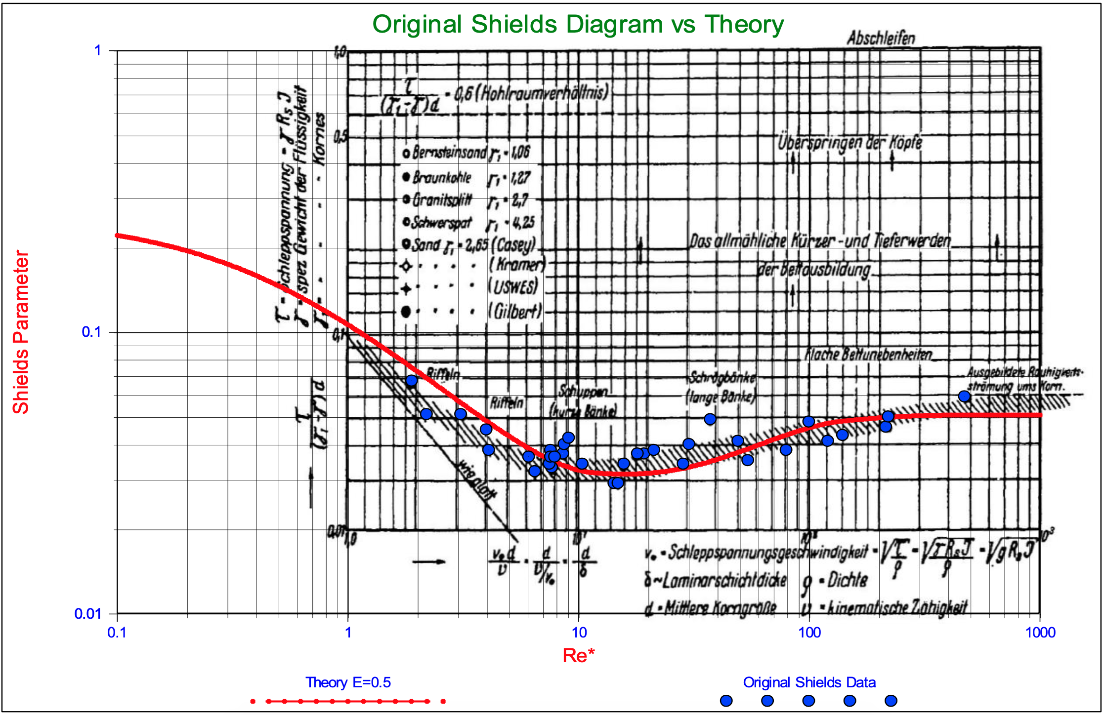
Although there may have been others before, Shields (1936) was one of the first who managed to give some physical explanation to the erosion phenomena and to found this with experiments. The results of his research are shown in Figure 5.1-1 together with the resulting theoretical curve from the current research. The original research as carried out by Shields in 1936 was based on a limited number of experiments and should be looked at in the context of the technology in that period. So it was and is a big achievement of Shields to find a relation for the initiation of motion of (spherical) particles that still holds today, although many have carried out additional research and tried to find a physical and mathematical explanation. These explanations usually incorporate phenomena such as gravity, drag, lift and turbulence and are based on sliding, rolling or lifting. Aspects such as, which velocity to use for the drag and the lift, where is the point of action of the drag force, the choice of the angle of repose and the pivoting angle are not always consistent. Especially the definition of incipient motion, is it when one particle starts moving, or many and then how many, is interpreted differently by different researchers. Some use sliding as the main mechanism, others rolling and a few lifting. Almost everybody uses the drag coefficient for spheres because many experiments are carried out for spheres, but real quarts grains have a larger drag coefficient especially at high Reynolds numbers. In general each of these models lacks one of these phenomena and/or aspects. The modeling usually stops, if a model has sufficient correlation with the data of many researchers (Buffington & Montgomery, 1997) and with the original Shields diagram (Shields, 1936).
5.1.1.1 Models on Sediment Threshold
Since there are many models available, only the most relevant ones, in the context of this book, will be discussed. Shields (1936) introduced the fundamental concepts for initiation of motion and made a set of observations (see Figure 5.1-1) that have become legendary. From dimensional analysis and fluid mechanics considerations he deduced the relation between the ratio of the bed shear stress and the gravitational force on a particle as a function of the boundary Reynolds number \(\ \mathrm{R} \mathrm{e} *=\mathrm{u} * \cdot \mathrm{d} /{v}_{\mathrm{l}}\). Based on curve fitting on his observations, the famous Shields curve was born. Later many experiments were carried out by numerous scientists of which Buffington & Montgomery give a nice summary (Buffington & Montgomery, 1997). Buffington also gives a critical analyses of the developments since Shields did his first findings (Buffington, 1999). In fact Shields did not derive a model or an equation, but published his findings as a graph (Figure 5.1-1). It is inconvenient that the Shields diagram is implicit, the friction velocity u* appears in both the horizontal and the vertical axis. However with modern computers this should not be any problem.
Although less famous, Hjulstrøm also carried out his research in the thirties (Hjulstrøm, 1935) and (Hjulstrøm, 1939). He presented his work in a graph showing the relation between the erosion velocity (average velocity above the bed) and the grain diameter. The graph, although explicit, depends on the water height, standard a height of 100 cm is used. For a certain water height, the Shields diagram can be converted to the Hjulstrøm diagram. A mathematical description of the Hjulstrøm diagram could not be found, but one will be given in the next paragraph. The equilibrium of a single particle resting on a granular bed was studied by White (1940). He obtained an expression for the threshold shear stress, but neglected the lift force. Later Kurihara (1948) extended the model and proposed some empirical equations for the estimation of threshold shear stress. Egiazaroff (1965) found a relation between the threshold shear stress and the particle Reynolds number. He assumed that at the moment of incipient motion the velocity at a height of 0.63·d is equal to the terminal settling velocity of the particle. His results did not match the original Shields data quantitatively, although some relation will exist.
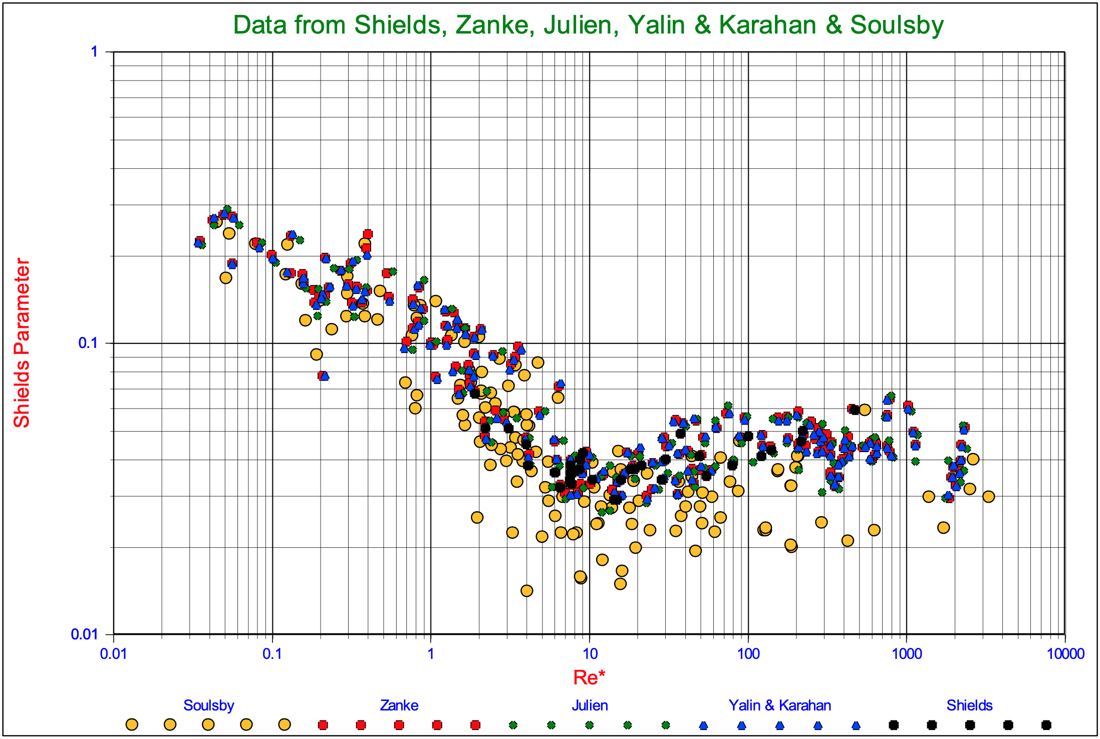
An extended Shields diagram was developed by Mantz (1977) followed by a graphical representation of a large volume of data by Yalin & Karahan (1979). The Ikeda-Coleman-Iwagaki model was presented by Ikeda (1982) and is based on the work of Iwagaki (1956) and Coleman (1967). The model is based on the assumption that the initiation of motion mechanism is sliding. Gravity, drag and lift are taken into account, but turbulence and grain placement are neglected. The zero level for the velocity profile is taken at the base of the grain exposed to the flow and the velocity used is at the center of the grain, so at y=d/2. This means that the grain is exposed to drag over the full height of the grain. For d/δv<0.5 the velocity profile of the viscous sub-layer is applied giving F(Re*)=u/u*=u*·d/(2·νl)=Re*/2, while for d/δv>2 the logarithmic velocity profile for rough boundaries is applied giving F(Re*)=u/u*=6.77. In the transition area, 0.5<d/δv<2 the fit for the velocity profile proposed by Swamee (1993) or Reichardt (1951) can be used by setting y=d/2 and ks=d. This leads to the following equation for the Shields parameter:
\[\ \mathrm{\theta=\frac{4}{3} \cdot \frac{\mu_{s f}}{C_{D}+\mu_{s f} \cdot C_{L}} \cdot \frac{1}{F\left(R e_{*}\right)^{2}}}\]
This equation is valid for horizontal beds, but the effect of a slope can easily be incorporated.
Considering two angles of internal friction (repose), φ=40°, (μsf=0.84) and φ=60°, (μsf=1.73) and further assuming that ks=2·d, CL=0.85·CD and using the standard relations for the drag coefficient for spheres, Garcia (2008) shows the resulting curves, compared with the original Shields (1936) data (Figure 5.1-1). The φ=40° curve underestimates the values of the Shields parameter compared with the original Shields data, while the φ=60° curve gets close, but still gives to small values. A φ=60° friction angle however is unreasonably high. The curve predicted follows the trend of Shields data, but is about a factor 1.6 smaller for the φ=40° case. A predecessor of this model was advanced by Egiazaroff (1965).
The Wiberg & Smith (1987A) model is based on the assumption that the initiation of motion mechanism is rolling. Gravity, drag and lift are taken into account and to some extend also turbulence. The equilibrium of moments around a pivot point is taken, where the location of the pivot point is defined as the contact point with an underlying particle under an angle \(\ \mathrm{\phi}\)0 with the vertical. This angle is named the particle angle of repose or the dilatation angle. This angle differs from the internal friction angle, as used in the Ikeda-Coleman-Iwagaki model, because the internal friction angle (angle of natural repose) is a global soil mechanical parameter, where local variations are averaged out, while the pivot angle is a local angle matching a specific configuration of the grains. The resulting Wiberg-Smith equation is almost equal to the Ikeda-Coleman-Iwagaki equation apart from the difference between the internal friction angle (using the friction coefficient) in equation (5.1-1) and the pivot angle in equation (5.1-2).
\[\ \mathrm{\theta=\frac{4}{3} \cdot \frac{\tan \left(\phi_{o}\right)}{C_{D}+\tan \left(\phi_{o}\right) \cdot C_{L}} \cdot \frac{1}{F\left(R e_{*}\right)^{2}}}\]
Wiberg & Smith (1987A) use the velocity profile as proposed by Reichardt (1951) providing a smooth transition between the viscous sub layer and the logarithmic profile. A lift coefficient of CL=0.2 is applied in the turbulent region, while it is assumed that particles residing completely in the viscous sub layer are not subject to lift. The calculations are carried out using \(\ \mathrm{\phi}\)0=50° and \(\ \mathrm{\phi}\)0=60° with ks=d. In Wiberg & Smith (1987B) the average velocity on the particle is applied, giving F(Re*)=6.0 for the hydraulic rough region. The model matches the original Shields data well for the turbulent rough region for \(\ \mathrm{\phi}\)0=60°, but overestimates the Shields data for the laminar flow in the viscous sub layer. The first conclusion does not come as a surprise, since \(\ \mathrm{\phi}\)0=60° is equal to μsf=1.73 in the Ikeda- Coleman-Iwagaki model and Wiberg & Smith use a smaller lift coefficient, resulting in a slightly higher curve. For the small Reynolds numbers the resulting curve overestimates the original Shields data. Wiberg & Smith (1987A) solve this by introducing turbulence. They state that periodic intrusions of high momentum liquid erode the viscous sub layer and produce locally higher boundary stresses. When the instantaneous boundary shear stress is sufficiently large, movement is more likely. To implement this the thickness of the viscous sub layer is reduced to 60%, maintaining the momentum of the flow, resulting in higher instantaneous velocities by a factor 1.66. This lowers the curve in the lower Reynolds area and gives a good match with the Shields data. This effect of turbulence however is the same for the whole lower Reynolds area and influences the asymptotic value of the Shields curve going to a Reynolds number of zero.
Dey (1999) developed a detailed model based on rolling as the mechanism for incipient motion. The model includes gravity, drag and lift and even Magnus lift forces, but no turbulence. The Morsi & Alexander (1972) relation for the drag coefficient is used, while the Saffman (1965) approach for the lift force is followed. Additionally the lift due to the Magnus effect is used for large Reynolds numbers. Based on detailed mathematics the lever arms for the equilibrium of moments are derived. The average velocity acting on the sphere is determined by integration of the velocity over the actual surface of the sphere, depending on the virtual bed level. The Reichardt (1951) velocity profile is used. The resulting equation for the Shields parameter is similar to equation (5.1-2), but much more detailed. There is an excellent agreement between the model developed by Dey and the experimental data used for a pivot angle of \(\ \mathrm{\phi}\)0=32°. For the particle considered, a particle resting on top of 3 other particles in a dense 3D configuration, the exposure level would be near 1.0 and the protrusion level near 0.8. The protrusion level is the fraction of a particle above the bed. The exposure level is the fraction of a particle exposed to the flow. Since the flow starts at about 20% of the particle diameter below the bed surface, the exposure level is about 0.2 higher than the protrusion level. According to a detailed study of Luckner (2002) this would result in a pivot angle of about \(\ \mathrm{\phi}\)0=20°.
Zanke (2001) and (2003) follows an approach different from all other researchers. Starting with a non-dimensional shear stress based on tilting a bed of particles and assuming that the shear stress exerted at the moment the top layer of the particles starts to move, he deducts the influences of turbulence and lift and finds a curve that is in good correlation with experimental data. The base non-dimensional shear stress is set to \(\ \theta\)=(1-n)·tan(φ/1.5), where the porosity n is set to 0.3 and the friction angle to \(\ \mathrm{\phi}\)0=30°. This starting point can be disputed since the driving force when tilting a bed until the grains start to move is gravity, while the main influence in initiation of motion is flow. The way turbulence is incorporated, both in drag and in lift is very interesting. The basis of the turbulence influences is the equation formulated by Nezu & Nakagawa (1993) for the turbulence intensity parallel to the wall as a function to the distance to the wall. Close to the wall in the viscous sub layer the turbulence intensity is about ur.m.s.+ =0.3·y +, where the time averaged velocity profile is known to be u+ =l·y+. Taking utotal+ =u+ +2.2·ur.m.s. =1.66·u+, should give the same result as Wiberg & Smith (1987A) found by reducing the thickness of the viscous sub layer to 60%. Zanke (2001) uses a factor of 1.8 instead of 2.2, but then his approach is completely different. Zanke (2001) must also have noticed that the asymptotic value of the curve for very low Reynolds numbers decreases when adding the influence of turbulence as stated above. Now it can be discussed whether the virtual bed level for the time averaged velocity and the turbulence intensity are exactly the same. By choosing a lower virtual bed level for the time averaged velocity, the ratio between the turbulence intensity and the time averaged velocity is zero at the virtual bed level for the turbulence intensity, resulting in an asymptotic value that is not influenced by the turbulence. Another interesting addition in the model of Zanke (2001) is the influence of cohesion, although it is the question which fundamental forces are taken into account.
Stevenson, Thorpe & Davidson (2002) and Stevenson, Cabrejos & Thorpe (2002) look at the process of incipient motion from the perspective of chemical engineering and also incorporated the rolling resistance. For small Reynolds numbers (viscous sub layer) the lift force is neglected.
It should be noted that a number of fit equations to the Shields data exist in order to be able to calculate the Shields parameter. A well know equation is the equation of Brownlie (1981) based on the Bonneville (1963) parameter D*.
\[\ \theta=\frac{0.22}{D_{*}^{0.9}}+0.06 \cdot e^{-17.77 \cdot D_{*}^{-0.9}}\]
Soulsby & Whitehouse (1997) defined another fit equation, based on the Bonneville (1963) parameter. The two fit equations differ in the asymptotic values. Brownlie uses 0.06 for very large Reynolds numbers, while Soulsby & Whitehouse use 0.055. As we will see later, this difference is not very relevant. The asymptote for very small Reynolds values for the Brownlie equation is proportional to D*-0.9, while Shields (1936) proposed 0.1 . D*-1, but Soulsby & Whitehouse found a value of 0.3, matching the mechanistic models as shown in the equations (5.1-1) and (5.1-2).
\[\ \theta=\frac{0.30}{\left(1+1.2 \cdot D_{*}\right)}+0.055 \cdot\left(1-e^{-0.02 \cdot D_{*}}\right)\]
Often it is found that for real sands and gravels the values found for initiation of motion (depending on the definition of course) are smaller than the ones found with the models and with the above equations. For this reason it is proposed to divide these equations by 2 for engineering purposes. Later we will see that this matches using the CD values for sands and gravels for large Reynolds numbers, but not for small Reynolds numbers.
5.1.1.2 Hjulström (1935), Sundborg (1956) and Postma (1967)
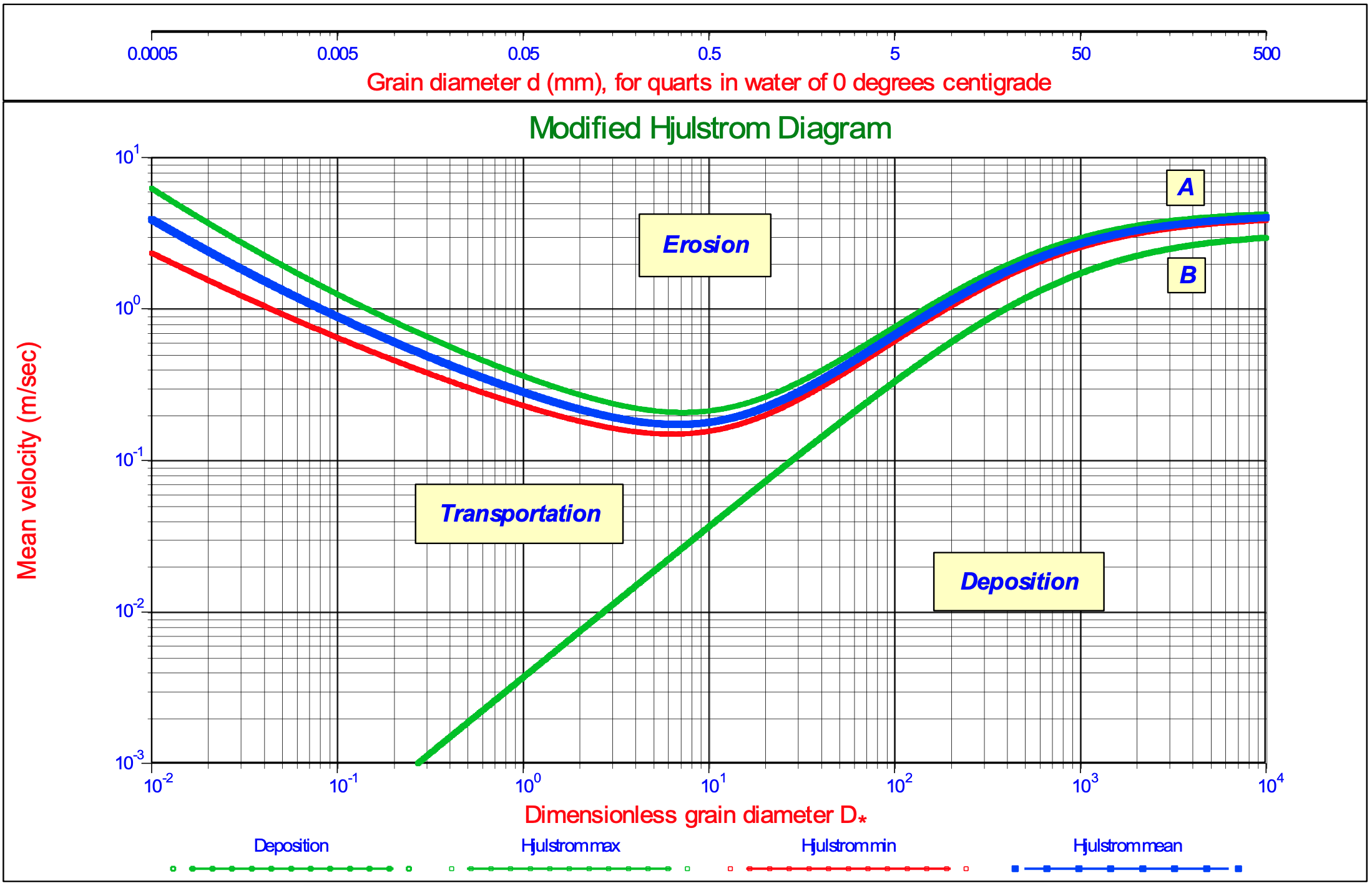
Although the Shields approach is used in this book, the following gives some background information. Hjulström (1935) & (1939) published the famous Hjulström diagram, showing the threshold flow velocity as a function of the particle diameter for a 100 cm water open channel flow. For large particles the threshold flow velocity increases with an increasing particle diameter, but for small particles the threshold flow velocity increases with a decreasing particle diameter. For particles near 0.5 mm a minimum threshold flow velocity is found. Figure 5.1-3 shows the Hjulström diagram. The increase of the threshold flow velocity with a decreasing particle diameter is explained with the phenomenon of cohesion. The research of Shields (1936) which was carried out in the same period of time did not contain such small particle diameters, thus cohesive effects were not included in this research. The Hjulström diagram can be well approximated with the following 2 empirical equations for the threshold flow velocity and the deposition velocity as derived by Miedema (2013).
\[\ \mathrm{U}_{\mathrm{c}}=\mathrm{1 . 5} \cdot\left(\frac{v_{\mathrm{l}}}{\mathrm{d}}\right)^{0.80}+\mathrm{0 . 8 5} \cdot\left(\frac{v_{\mathrm{I}}}{\mathrm{d}}\right)^{0.35}+9.5 \cdot \frac{\mathrm{R}_{\mathrm{sd}} \cdot \mathrm{g} \cdot \mathrm{d}}{\left(1+2.2 \mathrm{5} \cdot \mathrm{R}_{\mathrm{sd}} \cdot \mathrm{g} \cdot \mathrm{d}\right)}\]
\[\ \mathrm{U_{d}=77 \cdot \frac{d}{(1+24 \cdot d)}}\]
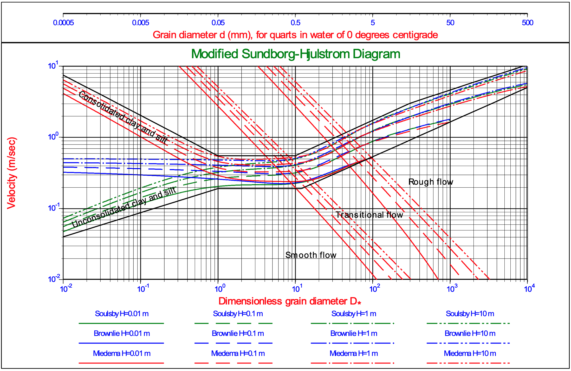
Sundborg (1956) modified the Hjulström diagram and included different levels of cohesion, resulting in a more or less constant threshold flow velocity in the absence of cohesive effects for small particle diameters and a similar behavior for cohesive soils. Postma (1967) further improved the diagram and talks about consolidated and unconsolidated soils. Figure 5.1-4 shows a modified Sundborg-Hjulström diagram. Later the research focused more on improving the modeling of the Shields diagram and finding experimental proof for this, resulting in a number of mechanistic models, as summarized by Buffington & Montgomery (1997) and Paphitis (2001), and a number of empirical equations of which the Brownlie (1981) equation and the Soulsby & Whitehouse (1997) equation should be mentioned. The Brownlie (1981) equation results in an increasing Shields value for a decreasing boundary Reynolds number with a power of almost -1. Translated into critical shear stress or shear velocity, this would result in an almost constant critical shear stress and shear velocity for a decreasing particle diameter. The Soulsby & Whitehouse (1997) equation results in an increasing shear stress and shear velocity for an increasing particle diameter for small particles. The shear stress increases almost linearly with the particle diameter and thus the shear velocity with the square root of the particle diameter. Figure 5.1-4 shows the behavior of both the Brownlie (1981) equation and the Soulsby & Whitehouse (1997) equation in the Sundborg-Hjulström diagram for 4 water depths. The third set of curves in this diagram are curves based on the Miedema (2012A) & (2012B) model, extended with the Zanke (2001) model for cohesion, as will be discussed later. From Figure 5.1-4 it is clear that unconsolidated soils (no cohesion) do not result in a horizontal line, but follow the Soulsby & Whitehouse (1997) equation, resulting in a proportionality between the threshold flow velocity and the particle diameter with a power of 0.5 for very small particles. The Brownlie (1981) equation gives a power of 0 and the Miedema (2010A) & (2010B) & Zanke (2001) model a power of -0.5 for cohesive soils. So the concept of a horizontal curve for unconsolidated/non-cohesive soils according to Sundborg (1956) and Postma (1967) is rejected here, instead the Soulsby & Whitehouse (1997) equation or the Miedema (2012A) & (2012B) model without cohesion should be used.
5.1.1.3 Shortcomings of the existing models
The existing models have developed during the years and have become more and more detailed. Still some shortcoming have been found and there is space for improvement.
- In general the exposure and protrusion levels used have not been well defined.
- When rolling is chosen as the mechanism for the initiation of motion, there is a relation between the protrusion level and the pivot angle and this cannot be chosen freely.
- The choice of rolling, sliding or lifting as the main mechanism for the initiation of motion has not been motivated well. It is very well possible that at high protrusion levels rolling will occur, while at low protrusion levels the mechanism is sliding and at protrusion levels around zero the mechanism is lifting. Looking at nature this does not sound unreasonable, since nature will choose the mechanism with the least resistance.
- All models use the relations for the drag coefficient for spheres, which is reasonable realizing that many experiments are carried out for spheres, but in reality we have to deal with natural sands and gravel, so the drag coefficient for sand should be used.
- The models do not incorporate rolling resistance which is reasonable since quarts is very hard and thus the rolling resistance is very low. Still it is interesting to investigate the influence of rolling resistance at very high protrusion levels.
- The models are not based on lifting, which is also reasonable, since it can be proven mathematically that initiation of motion by lifting requires a higher shear stress than rolling or sliding, so sliding or rolling will already occur before lifting could occur. Unless the bed is fixed and one single grain is subjected to the flow at a very low protrusion level.
- It is difficult to distinguish between the influence of drag and lift, since both are in the denominator of equations (5.1-1) and (5.1-2). Considering full turbulent flow resulting in drag and lift, while turbulence is phased out due to the size of the particles in relation with the size of the small turbulent eddies and considering laminar flow resulting in drag and the influence of small turbulent eddies, enables us to tune the model on the different physical phenomena.
- The models use the velocity at the center of the sphere, the average velocity on the sphere or the surface averaged velocity on the sphere. Also the lever arms for rolling are sometimes chosen at the center of the sphere or are determined by the surface averaged velocity. Since the forces on the sphere are determined by the square of the velocity in a linear or logarithmic velocity profile, the effective velocity should be determined by the surface averaged square of the velocity. This will give the actual acting point and lever arm.
- The models are based on velocity profiles and not on the effect of the velocity on the forces on the sphere. Turbulence is a stochastic process and turbulence intensity should not be treated as a velocity profile.
- The cross section for dragging and lifting is often chosen as the cross section of the sphere and thus chosen equal. The cross section for dragging sand lifting should depend on the protrusion and exposure levels and be different for dragging and lifting.
- Using a velocity profile in the transition between laminar and turbulent flow is dangerous, since it is not only the velocity that changes, but also the contributions of lift and turbulence and for example the position of the acting point of the drag force.
5.1.1.4 Knowns and Unknowns
The models identified with equations (5.1-1) and (5.1-2) contain a number of knowns and unknowns. The velocity profile and the drag coefficient can be determined theoretically or with semi-empirical equations. The viscosity (at a fixed temperature) and the Karman constant are known constants. The friction coefficient and the pivot angle can be found from many experiments or calculated geometrically. The main unknowns are the influence of turbulence and the influence of the lift coefficient. It is only useful to have different unknowns in a model if they can be isolated and measured independently. Looking at equations (5.1-1) and (5.1-2) we can see that both drag and lift are in the denominator and both drag and lift can be subject to the influence of turbulence, but then these influences cannot be isolated and measured separately. In general it can be assumed that lift does not occur in a laminar viscous flow, while the influence of small eddies is phased out for larger particles in a turbulent flow. So we will consider drag and turbulence for laminar viscous flow occurring at boundary Reynolds numbers below 5 and we will consider drag and lift for turbulent flow for boundary Reynolds numbers above 70. Since the drag based on the time averaged velocity profile is deterministic, this means that in the laminar viscous flow the only influence to make the model match the measurements is the turbulence, while in the turbulent flow the only influence to make the model match the measurements is the lift force. If there would be some lift force in the laminar viscous flow, the influence will be incorporated in the turbulence modelling, while a possible influence of turbulence in the turbulent region will be incorporated in the lift force modelling.
5.1.2 Velocity Distributions
In 2D open channel flow, usually a logarithmic velocity profile is assumed, with a very thin viscous sub layer near the bottom. Although the cross section of a pipe does not give a 2D profile, still most researchers use the 2D approach in their models.
5.1.2.1 Scientific Classification
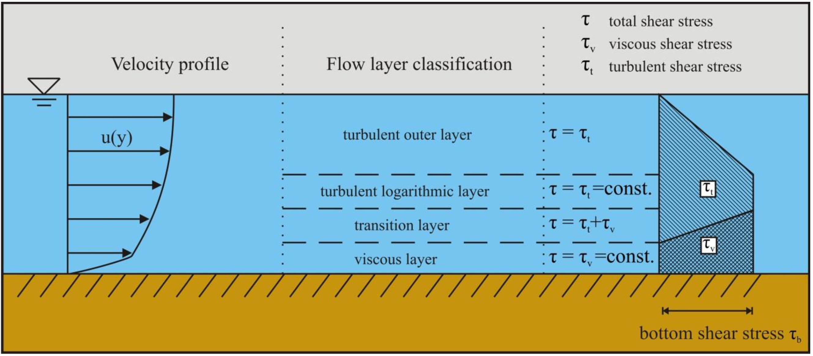
Figure 5.1-5 shows the classification of flow layers. Starting from the bottom we have:
- Viscous sub layer: a thin layer just above the bottom. In this layer there is almost no turbulence. Measurement shows that the viscous shear stress in this layer is constant. The flow is laminar. Above this layer the flow is turbulent.
- Transition layer: also called buffer layer, viscosity and turbulence are equally important.
- Turbulent logarithmic layer: viscous shear stress can be neglected in this layer. Based on measurement, it is assumed that the turbulent shear stress is constant and equal to bottom shear stress. It is in this layer where Prandtl introduced the mixing length concept and derived the logarithmic velocity profile.
- Turbulent outer layer: velocities are almost constant because of the presence of large eddies which produce strong mixing of the flow.
(Layer thickness is not to scale, turbulent outer layer accounts for 80% - 90% of the region).
5.1.2.2 Engineering Classification
In the turbulent logarithmic layer the measurements show that the turbulent shear stress is constant and equal to the bottom shear stress. By assuming that the mixing length is proportional to the distance to the bottom (l=κ·z), Prandtl obtained the logarithmic velocity profile.
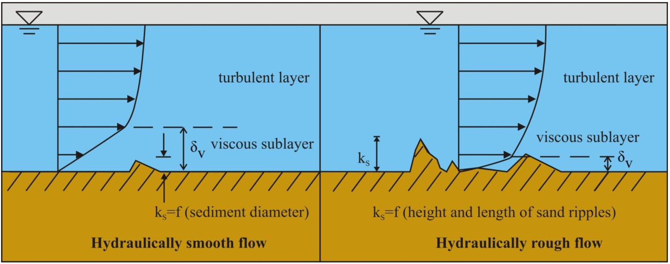
Various expressions have been proposed for the velocity distribution in the transitional layer and the turbulent outer layer. None of them are widely accepted. However, by the modification of the mixing length assumption, see next section, the logarithmic velocity profile applies also to the transitional layer and the turbulent outer layer. Measurement and computed velocities show reasonable agreement. Therefore from the engineering point of view, a turbulent layer with the logarithmic velocity profile covers the transitional layer, the turbulent logarithmic layer and the turbulent outer layer, see Figure 5.1-6.
As to the viscous sub layer, the effect of the bottom (or wall) roughness on the velocity distribution was first investigated for pipe flow by Nikuradse. He introduced the concept of equivalent grain roughness ks (Nikuradse roughness, bed roughness). Based on experimental data, it was found
- Hydraulically smooth flow for u*·ks/νl≤5, bed roughness is much smaller than the thickness of viscous sub layer. Therefore, the bed roughness will not affect the velocity distribution.
- Hydraulically rough flow for u*·ks/νl≥70, bed roughness is so large that it produces eddies close to the bottom. A viscous sub layer does not exist and the flow velocity is not dependent on viscosity.
- Hydraulically transitional flow for 5≤u*·ks/νl≤70, the velocity distribution is affected by bed roughness and viscosity.
5.1.2.3 Friction Velocity
The bottom shear stress is often represented by friction velocity, defined by:
\[\ \mathrm{u}_{*}=\sqrt{\frac{\tau_{\mathrm{b}}}{\rho_{\mathrm{l}}}}\]
The term friction velocity comes from the fact that \(\ \sqrt{\tau_{b} / \rho_{l}}\) has the same unit as velocity and it has something to do with friction force.
5.1.2.4 Turbulent Layer
In the turbulent layer the total shear stress contains only the turbulent shear stress. The total shear stress increases linearly with depth, i.e.
\[\ \tau_{t}(y)=\tau_{b} \cdot\left(1-\frac{y}{h}\right)\]
Expressed using Prandtl’s mixing length theory:
\[\ \tau_{\mathrm{t}}=\rho_{\mathrm{l}} \cdot \ell^{2}\left(\frac{\mathrm{d} \mathrm{u}}{\mathrm{dy}}\right)^{2}\]
Now assuming the mixing length is:
\[\ \ell=\mathrm{\kappa} \cdot \mathrm{y} \cdot\left(\mathrm{1}-\frac{\mathrm{y}}{\mathrm{h}}\right)^{\mathrm{0 . 5}}\]
With κ the Von Karman constant (κ=0.412) and h>>y, we get:
\[\ \frac{\mathrm{d u}}{\mathrm{d y}}=\frac{\mathrm{1}}{\mathrm{\kappa} \cdot \mathrm{y}} \cdot \sqrt{\frac{\tau_{\mathrm{b}}}{\rho}}=\frac{\mathrm{u}_{*}}{\mathrm{\kappa} \cdot \mathrm{y}}\]
Integration gives the famous logarithmic velocity profile (Law of the Wall):
\[\ \mathrm{u}(\mathrm{y})=\frac{\mathrm{u}_{*}}{\mathrm{\kappa}} \cdot \ln \left(\frac{\mathrm{y}}{\mathrm{y}_{0}}\right)\]
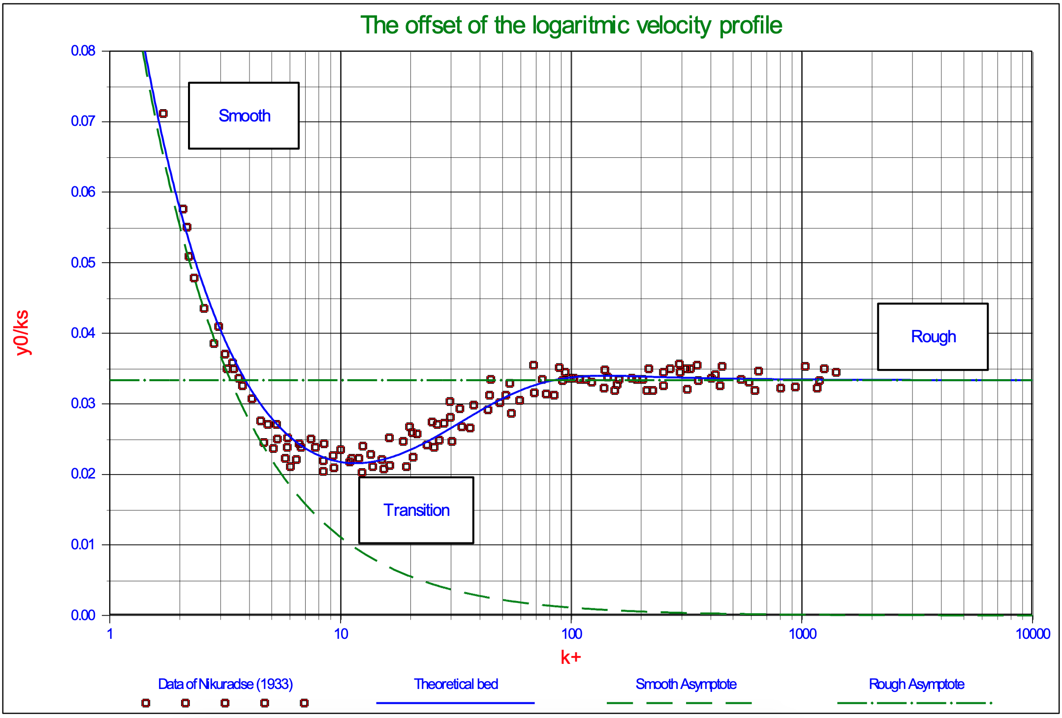
Where the integration constant y0 is the elevation corresponding to zero velocity (uy=y0=0), given by Nikuradse in his study of pipe flows.
\[\ \mathrm{y}_{\mathrm{0}}=\mathrm{0 . 1 1} \cdot \frac{v_{\mathrm{l}}}{\mathrm{u}_{*}} \quad\text{ Hydraulically smooth flow }\quad \frac{\mathrm{u}_{*} \cdot \mathrm{k}_{\mathrm{s}}}{v_{\mathrm{l}}} \leq \mathrm{5}\]
\[\ \mathrm{y}_{\mathrm{0}}=\mathrm{0 . 0 3 3} \cdot \mathrm{k}_{\mathrm{s}} \quad\text{ Hydraulically rough flow }\quad \frac{\mathrm{u}_{*} \cdot \mathrm{k}_{\mathrm{s}}}{v_{\mathrm{l}}} \geq \mathrm{7} \mathrm{0}\]
\[\ \frac{\mathrm{y}_{0}}{\mathrm{k}_{\mathrm{s}}}=\frac{1}{\mathrm{9} \cdot \mathrm{k}_{\mathrm{s}}^{+}}+\frac{1}{\mathrm{3 0}} \cdot\left(1-\mathrm{e}^{-\frac{\mathrm{k}_{s}^{+}}{26}}\right) \quad\text{ Hydraulically transition flow }\quad \mathrm{5}<\frac{\mathrm{u}_{*} \cdot \mathrm{k}_{\mathrm{s}}}{v_{\mathrm{l}}}<\mathrm{7} \mathrm{0}\]
5.1.2.5 Bed roughness
The bed roughness ks is also called the equivalent Nikuradse grain roughness, because it was originally introduced by Nikuradse in his pipe flow experiments, where grains are glued to the smooth wall of the pipes. The only situation where we can directly obtain the bed roughness is a flat bed consisting of uniform spheres, where ks = diameter of sphere. But in nature the bed is composed of grains with different size. Moreover, the bed is not flat, various bed forms, e.g. sand ripples or dunes, will appear depending on grain size and current. In that case the bed roughness can be obtained indirectly by the velocity measurement.
5.1.2.6 Viscous Sub-Layer
In the case of hydraulically smooth flow there is a viscous sub layer. Viscous shear stress is constant in this layer and equal to the bottom shear stress, i.e.
\[\ \tau_{v}=\rho_{1} \cdot v_{1} \cdot \frac{d u}{d y}=\tau_{b}\]
Integrating and applying uy=0=0 gives:
\[\ \mathrm{u}(\mathrm{y})=\frac{\tau_{\mathrm{b}}}{\rho_{\mathrm{l}}} \cdot \frac{\mathrm{y}}{v_{\mathrm{l}}}=\frac{\mathrm{u}_{*}^{2}}{v_{\mathrm{l}}} \cdot \mathrm{y}=\mathrm{y}^{+} \cdot \mathrm{u}_{*}\]
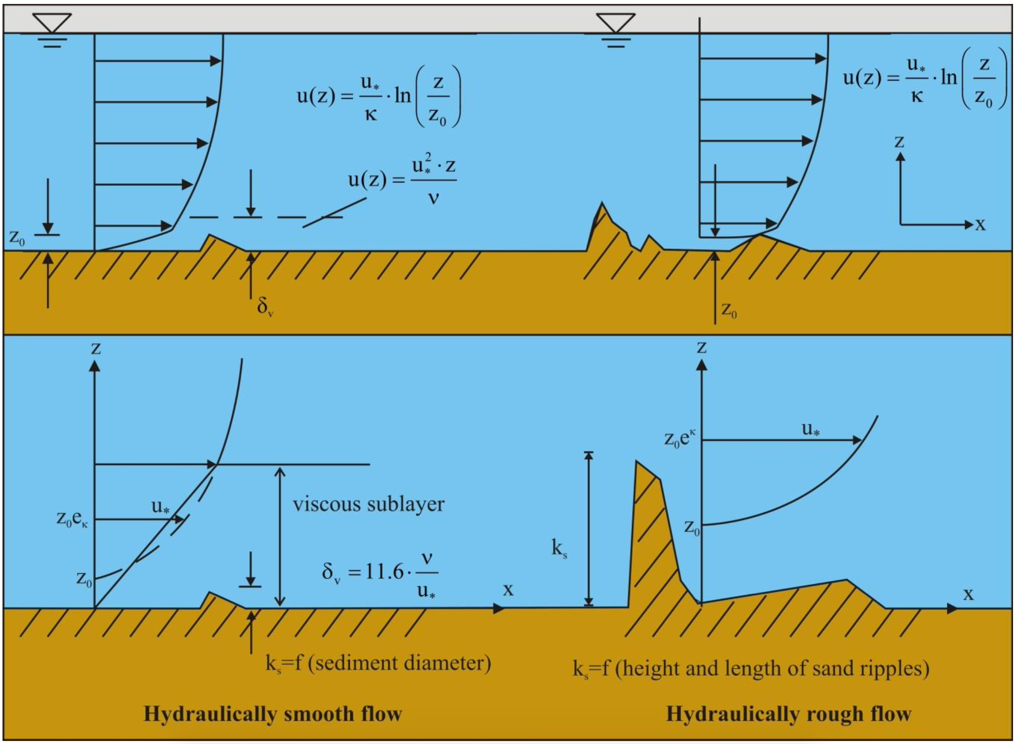
Thus, there is a linear velocity distribution in the viscous sub layer. The linear velocity distribution intersects with the logarithmic velocity distribution at the elevation y=11.6·νl/u*, yielding a theoretical viscous sub layer thickness δv:
\[\ \delta_{v}=11.6 \cdot \frac{v_{1}}{u_{*}}\]
The velocity profile is illustrated in Figure 5.1-8, with the detailed description of the fluid velocity near the bottom.
5.1.2.7 The Transition Laminar-Turbulent
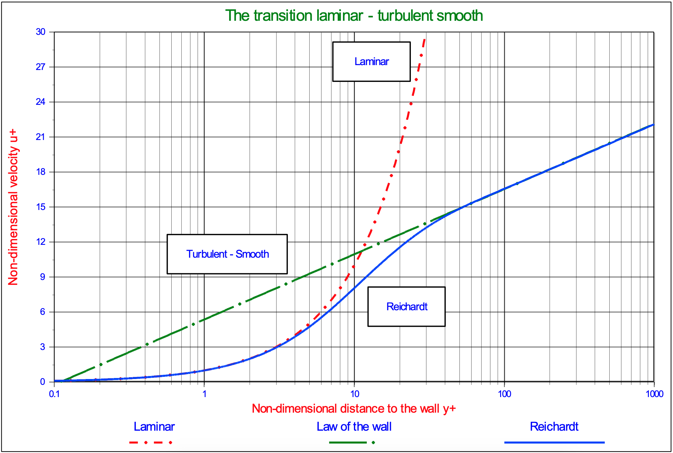
Reichardt (1951) derived an equation for the velocity that describes a laminar linear profile up to an y+ value of about 5, a turbulent logarithmic profile from an y+ value of about 40 and a transition velocity profile from 5 to 40 that is in excellent agreement with measurements made in that zone (see Schlichting (1968), p. 601). Equation (5.1-19) and Figure 5.1-9 show this velocity profile. Wiberg & Smith (1987A) and others also use this velocity profile.
\[\ \frac{\mathrm{u}(\mathrm{y})}{\mathrm{u}_{*}}=\frac{\ln \left(1+\mathrm{\kappa} \cdot \mathrm{y}^{+}\right)}{\mathrm{\kappa}}-\frac{\ln (\mathrm{1} / \mathrm{9})+\ln (\mathrm{\kappa})}{\mathrm{K}} \cdot\left(1-\mathrm{e}^{-\frac{\mathrm{y}^{+}}{11.6}}-\frac{\mathrm{y}^{+}}{\mathrm{1 1 . 6}} \mathrm{e}^{-\mathrm{0 . 3 3} \cdot \mathrm{y}^{+}}\right)\]
5.1.2.8 The Transition Smooth-Rough
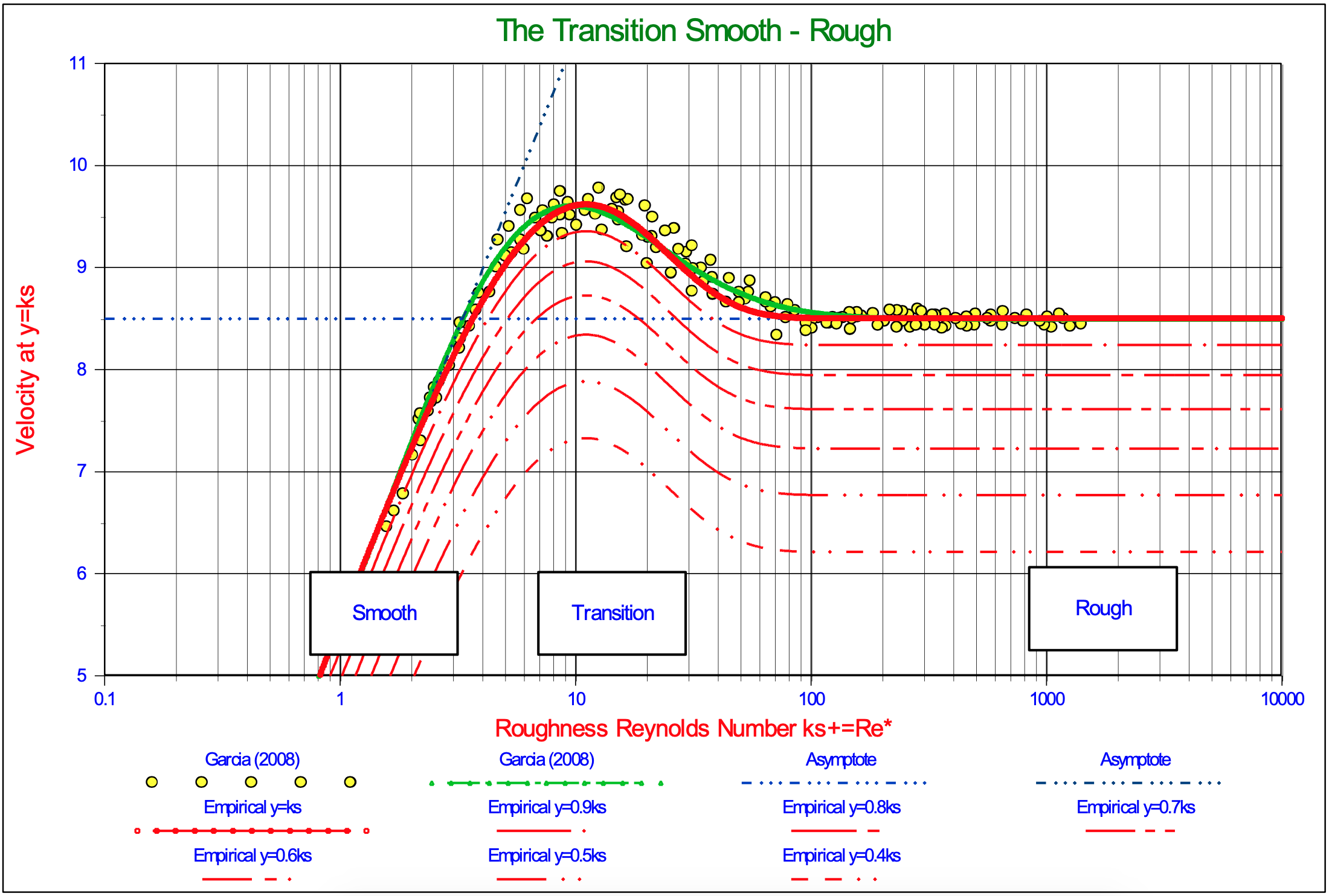
The transition between hydraulic smooth and rough flow can be approximated in many ways, but the resulting equation should match the measurements of Garcia (2008) (Figure 5.1-7). The following equation (derived by the author), give a very good approximation of this transition, where the distance to the wall equals the roughness. Equation (5.1-20) gives the velocity as a function of the non-dimensional distance to the wall y+.
\[\ \frac{\overline{\mathrm{u}}\left(\mathrm{y}^{+}\right)}{\mathrm{u}_{*}}=\frac{1}{\mathrm{\kappa}} \cdot \ln \left(\frac{\mathrm{y}^{+}}{\mathrm{0 . 1 1}}\right) \cdot \mathrm{e}^{-\mathrm{0 . 9 5} \cdot \frac{\mathrm{k}_{s}^{+}}{\mathrm{1 1 . 6}}}+\frac{1}{\mathrm{\kappa}} \cdot \ln \left(\frac{\mathrm{y}^{+}}{\mathrm{0 . 0 3 3} \cdot \mathrm{k}_{\mathrm{s}}^{+}}\right) \cdot\left(1-\mathrm{e}^{-\mathrm{0 . 9 5} \cdot \frac{\mathrm{k}_{s}^{+}}{11.6}}\right)\]
Since \(\ \mathrm{1 1} . \mathrm{6}=\mathrm{\delta}_{\mathrm{v}} \cdot \mathrm{u} * / v_{\mathrm{l}}=\mathrm{\delta}_{\mathrm{v}}^{+}\text{ and }\mathrm{0 . 1 1}=\mathrm{0 . 1 1} \cdot \mathrm{\delta}_{\mathrm{v}} \cdot \mathrm{u} * / v_{\mathrm{l}} / \mathrm{1 1} \mathrm{1 . 6}=\mathrm{0 . 0 0 9 5} \cdot \mathrm{\delta}_{\mathrm{v}^{+}}\) and the influence of the second right hand term (giving 95 instead of 105), equation (5.1-20) can be written as:
\[\ \frac{\overline{\mathrm{u}}\left(\mathrm{y}^{+}\right)}{\mathrm{u}_{*}}=\frac{1}{\mathrm{\kappa}} \cdot \ln \left(\mathrm{9 5} \cdot \frac{\mathrm{y}^{+}}{\delta_{\mathrm{v}}^{+}}\right) \cdot \mathrm{e}^{-\mathrm{0 . 9 5} \cdot \frac{\mathrm{k}_{\mathrm{s}}^{+}}{\delta_{\mathrm{v}}^{+}}}+\frac{\mathrm{1}}{\mathrm{\kappa}} \cdot \ln \left(\mathrm{3 0} \cdot \frac{\mathrm{y}^{+}}{\mathrm{k}_{\mathrm{s}}^{+}}\right) \cdot\left(1-\mathrm{e}^{-\mathrm{0 . 9 5} \cdot \frac{\mathrm{k}_{\mathrm{s}}^{+}}{\delta_{\mathrm{v}}^{+}}}\right)\]
In terms of the dimensional parameters for the distance to the wall y, the roughness ks and thickness of the laminar layer δv this gives:
\[\ \frac{\overline{\mathrm{u}}(\mathrm{y})}{\mathrm{u}_{*}}=\frac{1}{\mathrm{\kappa}} \cdot \ln \left(\mathrm{9 5} \cdot \frac{\mathrm{y}}{\delta_{\mathrm{v}}}\right) \cdot \mathrm{e}^{-\mathrm{0 . 9 5} \cdot \frac{\mathrm{k}_{\mathrm{s}}}{\delta_{\mathrm{v}}}}+\frac{\mathrm{1}}{\mathrm{\kappa}} \cdot \ln \left(\mathrm{3 0} \cdot \frac{\mathrm{y}}{\mathrm{k}_{\mathrm{s}}}\right) \cdot\left(1-\mathrm{e}^{-\mathrm{0 . 9 5} \cdot \frac{\mathrm{k}_{\mathrm{s}}}{\delta_{\mathrm{v}}}}\right)\]
Figure 5.1-10 shows the non-dimensional velocity u+ at distances y=ks, y=0.9·ks, y=0.8·ks, y=0.7·ks, y=0.6·ks, y=0.5·ks and, y=0.4·ks from the wall. Up to a Reynolds number of 20 and above a Reynolds number of 70 equation (5.1-20) matches the measurements very well, between 20 and 70 the equation underestimates the measured values, but overall the resemblance is very good.
5.1.3 The Model for Initiation of Motion
5.1.3.1 The Angle of Internal Friction/the Friction Coefficient
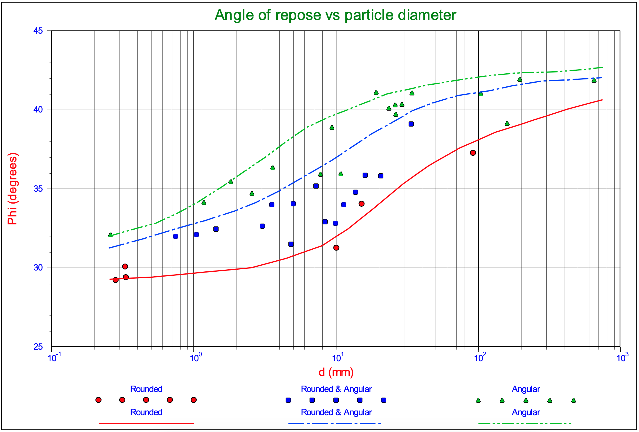
When the mechanism for the initiation of motion is sliding, friction is involved. The angle of repose of granular material is often referred to as the angle of internal friction of the material in a loose condition. By rotating a bed until the top layer of particles starts to move (slide or roll) the angle of repose is determined, which is the slope angle at that point. Another way of determining this angle is to pour the particles on a surface and measure the slope angle of the cone shaped heap of particles that is formed. In literature a value between 30°-35° is mentioned for natural sands. Figure 5.1-11 shows the angle of repose for different materials and grain sizes. The relation between the friction coefficient and the angle of repose is:
\[\ \mu_{\mathrm{sf}}=\tan (\phi)\]
It should be noted that the angle of repose, in this context, is a global soil mechanical parameter, which can be used as an average value when the whole top layer starts to move. Individual particles may encounter a different value. It should also be noted that the angle of repose is related to friction, which always has to do with the dissipation of energy, so it should not be mixed up with the pivot or dilatation angle which is related to resistance but not to the dissipation of energy.
5.1.3.2 The Pivot Angle/the Dilatation Angle
When the mechanism for the initiation of motion is rolling, a pivot angle is involved. For spheres there is a geometrical relation between the pivot angle and the protrusion level. The pivot angle is sometimes referred to as the dilatation angle, which however is a global soil mechanical parameter and it is preferred not to use it as a local parameter, so we will use the term pivot angle. Luckner (2002) (page 18) determined the pivot angle for 3D sphere configurations, from protrusion levels ranging from 0% to 82%. In fact the maximum protrusion level of a sphere on top of other spheres in a 3D configuration is 82%. At a protrusion level of 0%, meaning the sphere is in between and at the same level as the surrounding spheres, the pivot angle is ψ=90° At a protrusion level of 30% the pivot angle is ψ=59°, at 80% about ψ=20°, at 90% about ψ=12° and of course at 100% ψ=0°. In between these values a linear interpolation can be carried out. It is obvious that one is not free to choose the pivot angle, since it is related to the protrusion level.
Luckner (2002) determined the relation between the protrusion level and the pivot angle by using an ideal tetrahedral arrangement of spheres in a three dimensional approach. With the transformation from protrusion to exposure level and some curve fitting on the calculations of Luckner (2002), the following relation is found between the pivot angle ψ (in degrees) and the exposure level E, assuming the pivot angle equals the angle of contact as used here.
\[\ \psi=-144.12 \cdot \mathrm{E}^{4}+342.7 \cdot \mathrm{E}^{3}-245.05 \cdot \mathrm{E}^{2}-37.184 \cdot \mathrm{E}+104.28\]
5.1.3.3 The Lift Coefficient
The choice of the lift coefficient is a discussion in many of the models and many different values are found. Sometimes the lift coefficient is expressed as a fraction of the drag coefficient and sometimes as a constant. In most models however lift is present in the turbulent flow, but not in the laminar viscous sub layer. In this model also the choice is made to neglect lift in the laminar region, so for boundary Reynolds numbers below 5. Wiberg & Smith (1987A), Dey (1999), Pilotti & Menduni (2001), Stevenson, Thorpe & Davidson (2002) and others support this assumption. For the turbulent region different values are used for the lift coefficient.
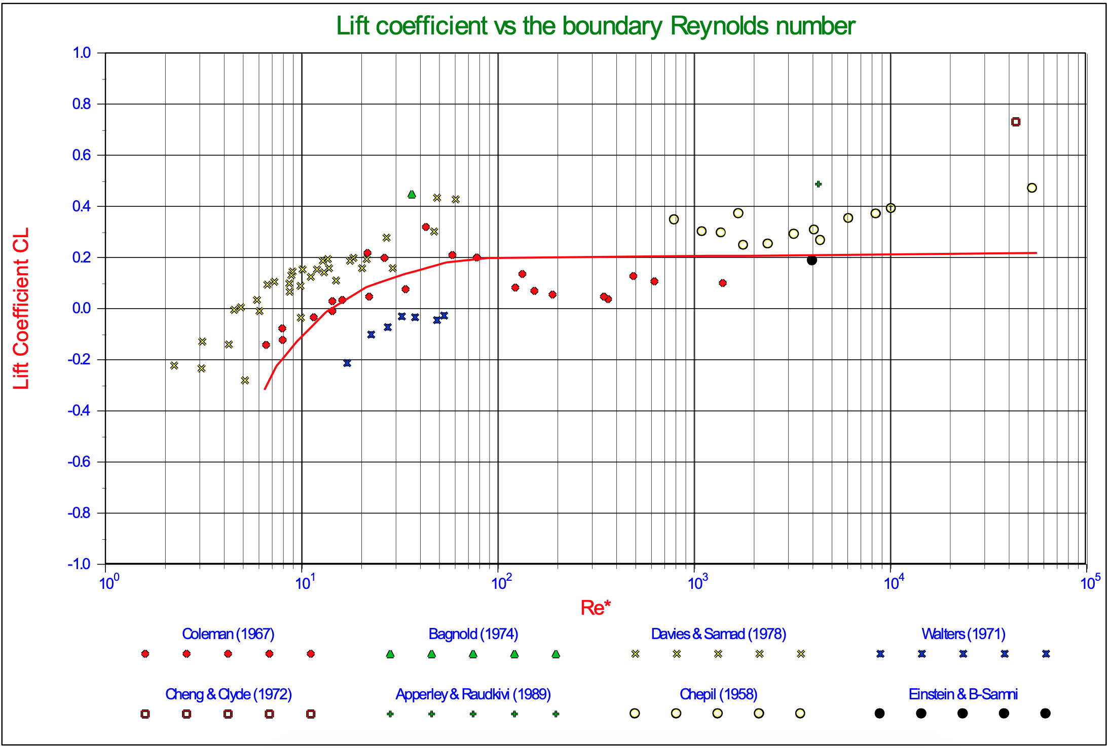
Wiberg & Smith (1987A) use a value of 0.2, while using 0.85·CD in (Wiberg & Smith, 1987B) inspired by the work of Chepil (1958). Marsh, Western & Grayson (2004) compared 4 models, but also evaluated the lift coefficient as found by a number of researchers as is shown in Figure 5.1-12. For large Reynolds numbers an average value of 0.2 is found, while for small Reynolds numbers the lift coefficient can even become negative. Luckner (2002) found a relation where the lift coefficient is about 1.9·E·CD (including the effect of turbulence), which matches the findings of Dittrich, Nestmann & Ergenzinger (1996). For an exposure level of 0.5 this gives 0.95·CD which is close to the findings of Chepil (1958). Using a lift coefficient of 0.95·CD=0.423 for boundary Reynolds numbers above 70, results in Shields curves matching the experimental data.
5.1.3.4 Turbulence
Turbulence describes the stochastic non-deterministic velocity fluctuations in a flow and although coherent structures exist in the occurrence of turbulence, turbulence has no long term memory. The implication of this is that turbulence cannot be described by a velocity profile, but instead it can be described by statistical properties. In general it is described by the turbulence intensity of the horizontal and vertical velocity and the intensity of the Reynolds stress. These intensities reflect the so called r.m.s. (root mean square) values of the velocity fluctuations. Assuming the velocity fluctuations are according to a normal or Gaussian distribution, the time and surface averaged velocity profiles represent the mean value of the distribution, as used in equations (5.1-19) and (5.1-21), while the standard deviation is represented by the r.m.s. value, also called the first moment of the distribution. The second moment and third moment correspond to two times and three times the r.m.s. value. The probability of having an instantaneous velocity higher than the standard deviation in the direction of the mean velocity is 14.9%, for the second moment this is 2.3% and for the third moment 0.13%.
Wiberg & Smith (1987A) reduce the height of the viscous sub layer to 60%, resulting in an increase of 1/0.6=1.66 of the velocity in the viscous sub layer. Assuming a turbulence intensity of 0.3·y+·u* (Nezu & Nakagawa, 1993) and a mean velocity of y+·u*, implicitly this means adding 2.2 times the turbulence intensity to the mean velocity. Since Wiberg & Smith only apply this for low boundary Reynolds numbers where the particles are small with regard to the height of the viscous sub layer, implicitly this means adding a turbulence effect to small boundary Reynolds numbers (smooth boundaries) and not to large boundary Reynolds numbers (rough boundaries). Hofland (2005) in his PhD thesis states that fluctuations created by smaller eddies are negligible for larger particles due to phase cancellations when integrated over the surface of a stone. Zanke (2001) and later Luckner (2002) apply turbulent velocity fluctuations both for small and large boundary Reynolds numbers and add 1.8 times the turbulence intensity to the mean velocity. Nezu & Nakagawa (1977) and (1993) and Nezu & Rodi (1986) found the following relation for the turbulence intensity parallel to the wall.
\[\ \frac{\mathrm{u}_{\mathrm{r} . \mathrm{m} . \mathrm{s} .}}{\mathrm{u}_{*}}=\mathrm{0 . 3} \cdot \mathrm{y}^{+} \cdot \mathrm{e}^{-\frac{\mathrm{y}^{+}}{\mathrm{1 0}}}+\mathrm{2 . 2 6 \cdot e}^{-\frac{\mathrm{y}}{\mathrm{h}}} \cdot\left(\mathrm{1 - e}^{-\frac{\mathrm{y}^{+}}{\mathrm{1 0}}}\right)\]
The asymptotic value of the ratio between the turbulence intensity and the time and surface averaged velocity is 0.3. Measurements of this ratio, carried out by Eckelman (Hinze, 1975) on smooth walls as a function of the distance to the wall y+, show a small increase near the wall to a value of 0.38 at y+ =4. Approaching the wall further shows a decrease to a value of 0.24, but the measurements do not contradict the assumption of having a ratio at the wall of zero. Kim, Moin and Moser (1987) confirm these findings, but state that additional measurements show a finite value at the wall, although the measurements in their paper do not contradict a value of zero. Zanke (2003) assumes a ratio of zero at the wall and achieves this by shifting the time averaged velocity with respect to the distance to the wall. In fact implicitly this means that the virtual bed level for the time averaged velocity (which is chosen at 0.2·d below the top of the spheres in this paper) is located lower than the virtual bed level for the turbulence intensity.
Considering that the measurements of Eckelman and later Kim, Moin & Moser were carried out on a smooth wall where the wall is the virtual bed level, while here we consider a bed of grains or spheres where a virtual bed level has to be defined, resulting in a correct drag force on the spheres, there is no reason why the two virtual bed levels should be the same. The solution of Zanke, choosing two different virtual bed levels is one way of solving this problem. One can also choose one virtual bed level for both, the time averaged velocity and the turbulence intensity, but consider that below the top of the spheres, the turbulence intensity is decreased, due to the shadow effect of the spheres. Assuming the turbulence intensity to be zero at the virtual bed level and increasing proportional to the square of the distance to the wall, very close to the wall between the grains, and proportional to the distance to the wall above the grains, this can be represented with the following equation:
\[\ \frac{\mathrm{u}^\prime_{\mathrm{r} . \mathrm{m} . \mathrm{s} .}}{\mathrm{u}_{*}}=\frac{\mathrm{u}_{\mathrm{r} . \mathrm{m} . \mathrm{s} .}}{\mathrm{u}_{*}} \cdot\left(\mathrm{1}-\mathrm{e}^{-\mathrm{y}^{+}}\right)\]
Another reason for assuming a ratio of zero at the virtual bed level is the fact that the asymptotic value found for the Shields curve for the boundary Reynolds number approaching zero matches the measurements (see Figure 5.1-15). Any ratio larger than zero would lower the curves found. Figure 5.1-13C shows the turbulence intensity according to equation (5.1-25), while Figure 5.1-13A shows the turbulence intensity very close to the wall. Figure 5.1-13B shows the difference between equation (5.1-25) and applying damping on the turbulence intensity very close to the wall according to equation (5.1-26). The turbulence intensity profile according to equation (5.1-26) does not contradict the findings of Nezu and Nakagawa (1993), Eckelman (Hinze, 1975) and Kim, Moin & Moser (1987) and matches the findings of Zanke (2003). Now it is the question how many times the standard deviation of the turbulence intensity should be used.
Wiberg & Smith (1987A) implicitly used a factor 2.2 and Zanke (2003) used a factor 1.8 explicitly. Since we consider the initiation of motion, particles or spheres will start to entrain if there is one moment when the condition for entrainment is satisfied. On the other hand the Shields curve falls somewhere between critical and general transport, meaning that already many particles at many locations entrain. The factor n in equation (5.1-27), the turbulence intensity factor, is chosen 3. Meaning that the probability of having a higher instantaneous velocity is only 0.13%, so about 1 out of 1000 occurrences of turbulent eddies.
\[\ \frac{\mathrm{u}^\prime_{\mathrm{n} \cdot \mathrm{r} . \mathrm{m} . \mathrm{s} .}}{\mathrm{u}_{*}}=\mathrm{n} \cdot \frac{\mathrm{u}_{\mathrm{r} . \mathrm{m} . \mathrm{s}}^{\prime}}{\mathrm{u}_{*}}\]
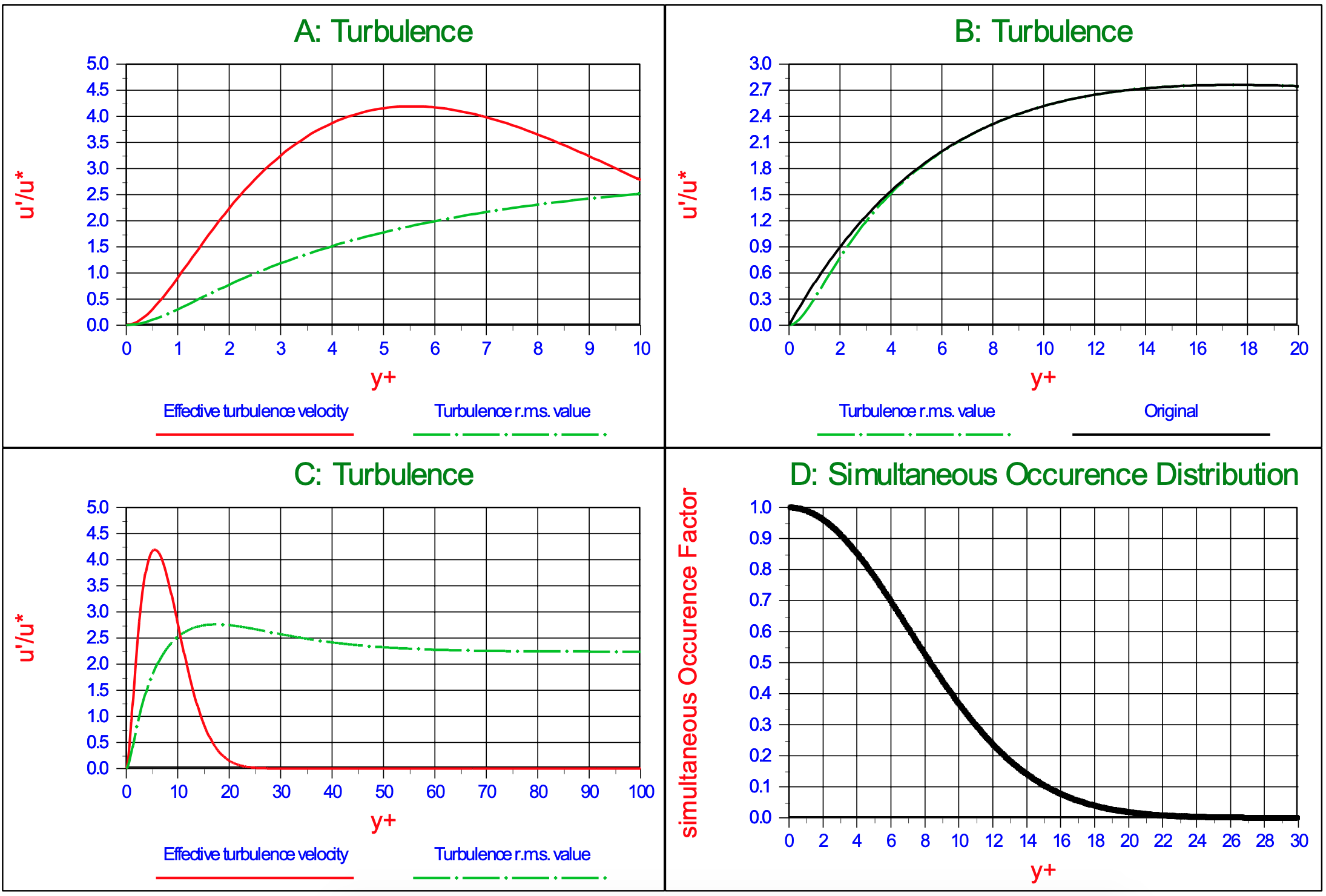
The resulting turbulence intensity profile should not be interpreted as a velocity distribution, since it describes the intensity of stochastic turbulent velocity fluctuations. This means that the influence of these fluctuations on the drag force can be derived by integrating the fluctuations over the height of a particle and in fact this should be added to the mean velocity and then the surface averaged value of the square of the total velocity should be determined. Taking the square root of this velocity and deducting the time averaged velocity gives the contribution of the turbulence. Since at one location the turbulent velocity fluctuations will be positive, while at the same time at other locations they will be negative, the probability that at one moment in time the turbulent velocity fluctuations over the height of the particle are unidirectional in the direction of the time averaged velocity is almost zero.
For very small particles having a diameter smaller than or equal to the size of the small turbulent eddies, this may still be the case, but with increasing diameter the influence of the eddies will decrease due to the fact that they cancel each other out. For very large particles the influence of this turbulence will reduce to zero. It is proposed to name this effect the probability of simultaneous occurrence effect and the factor determining the turbulent velocity that should be added to the time averaged velocity, the factor of simultaneous occurrence. The point of action of the resulting surface averaged square of the velocity is assumed not to change, although there is no reason for that.
With the height y+=E·Re* at the top of a particle with exposure level E, equation (5.1-28) is proposed for the factor of simultaneous occurrence and this is shown in Figure 5.1-13D. The resulting effective velocity profile is shown in Figure 5.1-13C and Figure 5.1-13A.
\[\ \frac{\mathrm{u}_{\mathrm{eff}}}{\mathrm{u}_{*}}=\frac{\mathrm{u}_{\mathrm{n} \cdot \mathrm{r} . \mathrm{m} . \mathrm{s} .}}{\mathrm{u}_{*}} \cdot \mathrm{e}^{-\left(\frac{\mathrm{y}^{+}}{\mathrm{1 0}}\right)^{2}}\]
5.1.3.5 Approach
Before developing the model a number of assumptions have to be made in order to have starting points for the modeling to match the Shields curve and the measurements from literature. These assumptions have to be reasonable, matching literature and practice. These assumptions are:
- The bed consists of spheres with one diameter d.
- The virtual bed level is chosen at 0.2·d below the top of the bed.
- The criterion for initiation of motion is chosen to be between critical transport and general transport according to Vanoni (1975), Delft Hydraulics (1972) and Graf & Pazis (1977).
- The exposure level E is chosen as 0.5·d, resulting in a protrusion level of 0.3·d, meaning that the standard sphere is exposed to the flow for 50% and reaches above the other spheres in the bed for 30%, based on Fenton & Abbot (1977) and Chin & Chiew (1993).
- For the model an internal friction angle (angle of natural repose) of φ=30° is chosen (for the sliding mechanism), which matches spheres and rounded particles of natural sands and gravel (see Figure 5.1-11).
- For the model a pivot angle of ψ=59° is chosen (for the rolling mechanism), which matches a protrusion level of 0.3·d, based on Luckner (2002).
- First full laminar flow will be considered up to a boundary/roughness Reynolds number of 11.6 and full turbulent flow above 11.6. The laminar flow is described with equation (5.1-19) and the turbulent flow with equation (5.1-17).
- Later a transition area is introduced with full laminar flow up to a boundary/roughness Reynolds number of 5, a transition zone from 5 to 70 and a full turbulent flow above 70, with logarithmic interpolation in the transition zone.
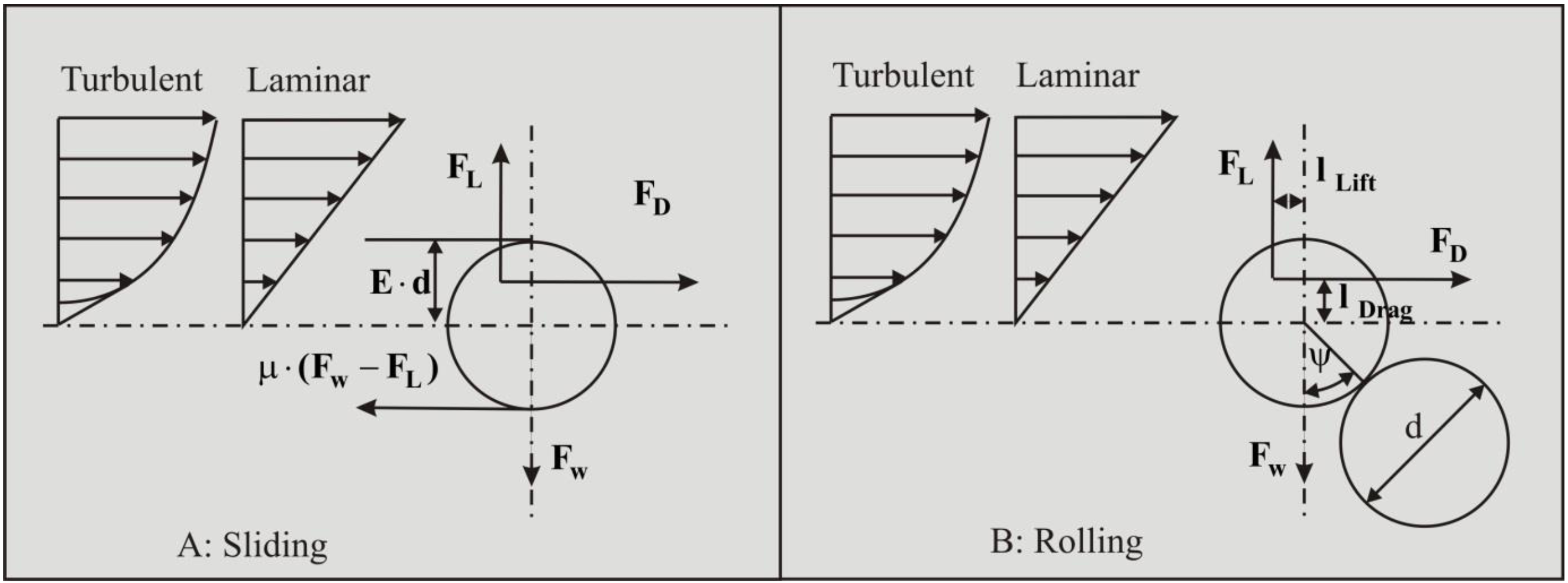
- For the laminar flow, the velocity at the top of the sphere is 0.5·Re*·u*, resulting in an acting point at $\ell_{\text {Drag }}$=0.5, meaning at 50% of the flow field (see equation (5.1-19)). This also means the acting point is at 0.25·d above the center of the sphere (based on a surface averaged square of the velocity).
- For the turbulent flow, the velocity at the top of the sphere is ln(0.5/0.033)·u*/κ=6.6·u*,resulting in an acting point at \(\ \ell_{\mathrm{Drag}}=\mathrm{0 . 6 5 5}\), meaning at 65.5% of the flow field (see equation (5.1-12)). This also means the acting point is at 0.327·d above the center of the sphere (based on a surface averaged square of the velocity).
In Miedema (2012A) & (2012B), a model for the entrainment of particles as a result of liquid (or air) flow over a bed of particles has been developed based on the above assumptions. The model distinguishes sliding, rolling and lifting as the mechanisms of entrainment. Sliding is a mechanism that occurs when many particles are starting to move and it is based on the global soil mechanical parameter of internal friction. Both rolling and lifting are mechanisms of individual particles and they are based on local parameters such as the pivot angle and the exposure and protrusion rate. Equations (5.1-34), (5.1-38) and (5.1-42) give the Shields parameter for these 3 mechanisms.
5.1.3.6 Drag and Lift Induced Sliding
Let us consider the steady flow over a bed composed of cohesion less grains. The driving forces are the flow drag and lift forces on the grain, assuming that part of the surface of the particle is hiding behind other particles and only a fraction E (the exposure level) is subject to drag and lift. This gives the following equation for the drag force:
\[\ \mathrm{F}_{\mathrm{D}}=\mathrm{C}_{\mathrm{D}} \cdot \frac{1}{2} \cdot \rho_{\mathrm{l}} \cdot\left(\ell_{\mathrm{D r a g}} \cdot \mathrm{\alpha} \cdot \mathrm{u}_{*}\right)^{2} \cdot \mathrm{f}_{\mathrm{D}} \cdot \frac{\pi \cdot \mathrm{d}^{2}}{4}\]
The lift force is written in the same way, but it is assumed that the lift force is determined by the velocity difference between the top and the bottom of the particle and the surface that is subject to lift is the projected horizontal cross section subject to the flow, this factor fL=1 for an exposure level E=0.5, while the factor for drag fD=0.5 in this case:
\[\ \mathrm{F}_{\mathrm{L}}=\mathrm{C}_{\mathrm{L}} \cdot \frac{1}{2} \cdot \rho_{\mathrm{l}} \cdot\left(\mathrm{\alpha} \cdot \mathrm{u}_{*}\right)^{2} \cdot \mathrm{f}_{\mathrm{L}} \cdot \frac{\pi \cdot \mathrm{d}^{2}}{\mathrm{4}}\]
The submerged weight of the particle is:
\[\ \mathrm{F}_{\mathrm{w}}=\left(\rho_{\mathrm{q}}-\rho_{\mathrm{l}}\right) \cdot \mathrm{g} \cdot \frac{\pi \cdot \mathrm{d}^{\mathrm{3}}}{6}\]
At equilibrium the drag force and the friction force are equal (note that the friction force is reduced by the lift):
\[\ \mathrm{F}_{\mathrm{D}}=\boldsymbol{\mu}_{\mathrm{s f}} \cdot\left(\mathrm{F}_{\mathrm{w}}-\mathrm{F}_{\mathrm{L}}\right)\]
Substituting the equations (5.1-29), (5.1-30) and (5.1-31) into (5.1-32) results in the following equation:
\[\ \mathrm{C}_{\mathrm{D}} \cdot \frac{1}{2} \cdot \rho_{\mathrm{l}} \cdot\left(\ell_{\mathrm{D r a g}} \cdot \mathrm{\alpha} \cdot \mathrm{u}_{*}\right)^{2} \cdot \mathrm{f}_{\mathrm{D}} \cdot \frac{\pi \cdot \mathrm{d}^{2}}{\mathrm{4}}=\mu_{\mathrm{sf}} \cdot\left(\left(\rho_{\mathrm{q}}-\rho_{\mathrm{l}}\right) \cdot \mathrm{g} \cdot \frac{\pi \cdot \mathrm{d}^{3}}{\mathrm{6}}-\mathrm{C}_{\mathrm{L}} \cdot \frac{1}{2} \cdot \rho_{\mathrm{l}} \cdot\left(\mathrm{\alpha} \cdot \mathrm{u}_{*}\right)^{2} \cdot \mathrm{f}_{\mathrm{L}} \cdot \frac{\pi \cdot \mathrm{d}^{2}}{\mathrm{4}}\right)\]
Which can be re-arranged into (showing the Shields parameter):
\[\ \theta_{\text {sliding }}=\frac{\mathrm{u}_{*}^{2}}{\mathrm{R}_{\mathrm{s d}} \cdot \mathrm{g} \cdot \mathrm{d}}=\frac{\mathrm{4}}{\mathrm{3}} \cdot \frac{\mathrm{1}}{\alpha^{2}} \cdot \frac{\mu_{\mathrm{s f}}}{\ell_{\mathrm{D r a g}}^{2} \cdot \mathrm{f}_{\mathrm{D}} \cdot \mathrm{C}_{\mathrm{D}}+\mu_{\mathrm{s f}} \cdot \mathrm{f}_{\mathrm{L}} \cdot \mathrm{C}_{\mathrm{L}}}\]
5.1.3.7 Drag and Lift Induced Rolling
The equilibrium equation for rolling is:
\[\ \mathrm{F}_{\mathrm{D}} \cdot\left(\ell_{\mathrm{L} \mathrm{e v e r}-\mathrm{D}}+\cos \left(\psi+\phi_{\mathrm{Roll} }\right)\right) \cdot \mathrm{R}+\mathrm{F}_{\mathrm{L}} \cdot\left(\ell_{\mathrm{L} \operatorname{ever}-\mathrm{L}}+\sin \left(\psi+\phi_{\mathrm{Roll}}\right)\right) \cdot \mathrm{R}=\mathrm{F}_{\mathrm{w}} \cdot \sin \left(\Psi+\phi_{\mathrm{Roll}}\right) \cdot \mathrm{R}\]
Substituting the equations (5.1-29), (5.1-30) and (5.1-31) into (5.1-35) gives:
\[\ \mathrm{C}_{\mathrm{D}} \cdot \frac{1}{2} \cdot \rho_{\mathrm{l}} \cdot\left(\ell_{\mathrm{D r a g}} \cdot \mathrm{\alpha} \cdot \mathrm{u}_{*}\right)^{2} \cdot \mathrm{f}_{\mathrm{D}} \cdot \frac{\pi \cdot \mathrm{d}^{2}}{\mathrm{4}} \cdot\left(\ell_{\mathrm{L} \operatorname{ever}-\mathrm{D}}+\cos \left(\psi+\phi_{\mathrm{Roll}}\right)\right) \cdot \mathrm{R}
+\mathrm{C}_{\mathrm{L}} \cdot \frac{1}{2} \cdot \rho_{\mathrm{l}} \cdot\left(\mathrm{\alpha} \cdot \mathrm{u}_{*}\right)^{2} \cdot \mathrm{f}_{\mathrm{L}} \cdot \frac{\pi \cdot \mathrm{d}^{2}}{\mathrm{4}} \cdot\left(\ell_{\mathrm{L} \operatorname{ever}-\mathrm{L}}+\sin \left(\psi+\phi_{\mathrm{Roll}}\right)\right) \cdot \mathrm{R}
=\left(\rho_{\mathrm{q}}-\rho_{\mathrm{l}}\right) \cdot \mathrm{g} \cdot \frac{\boldsymbol{\pi} \cdot \mathrm{d}^{\mathrm{3}}}{\mathrm{6}} \cdot \sin \left(\psi+\phi_{\mathrm{Roll}}\right) \cdot \mathrm{R} \]
With the additional lever arms for drag and lift:
\[\ \begin{array}\ell_{\text {Lever- } \mathrm{D}}=1-2 \cdot \mathrm{E} \cdot\left(1-\ell_{\text {Drag }}\right)\\
\ell_{\text {Lever-L }}=0\end{array}\]
Which can be re-arranged into the Shields parameter:
\[\ \theta_{\text {rolling }}=\frac{\mathrm{u}_{*}^{2}}{\mathrm{R}_{\mathrm{s d}} \cdot \mathrm{g} \cdot \mathrm{d}}=\frac{\mathrm{4}}{\mathrm{3}} \cdot \frac{\mathrm{1}}{\alpha^{2}} \cdot \frac{\mu_{\mathrm{r f}}}{\ell_{\mathrm{D r a g}}^{2} \cdot \mathrm{f}_{\mathrm{D}} \cdot \mathrm{C}_{\mathrm{D}}+\mu_{\mathrm{r f}} \cdot \mathrm{f}_{\mathrm{L}} \cdot \mathrm{C}_{\mathrm{L}}}\]
With the effective rolling friction coefficient \(\ \mu_{\mathrm{rf}}\) :
\[\ \mu_{\mathrm{rf}}=\frac{\sin \left(\psi+\phi_{\mathrm{Roll}}\right)}{\ell_{\mathrm{Lever}-\mathrm{D}}+\cos \left(\psi+\phi_{\mathrm{Roll}}\right)}
\]
5.1.3.8 Lift Induced Lifting
A third possible mechanism for the initiation of motion is pure lifting. This will occur if the lift force is equal to the gravity force according to:
\[\ \mathrm{F}_{\mathrm{w}}=\mathrm{F}_{\mathrm{L}}\]
Substituting the equations (5.1-29) and (5.1-31) into equation (5.1-40) gives:
\[\ \left(\rho_{\mathrm{s}}-\rho_{\mathrm{l}}\right) \cdot \mathrm{g} \cdot \frac{\pi \cdot \mathrm{d}^{3}}{6}=\mathrm{C}_{\mathrm{L}} \cdot \frac{1}{2} \cdot \rho_{\mathrm{l}} \cdot\left(\alpha \cdot \mathrm{u}_{*}\right)^{2} \cdot \mathrm{f}_{\mathrm{L}} \cdot \frac{\pi \cdot \mathrm{d}^{2}}{4}\]
Which can be re-arranged into the Shields parameter:
\[\ \theta_{\text {lifting }}=\frac{\mathrm{u}_{*}^{2}}{\mathrm{R}_{\text {sd }} \cdot \mathrm{g} \cdot \mathrm{d}}=\frac{4}{3} \frac{1}{\alpha^{2} \cdot \mathrm{C}_{L} \cdot \mathrm{f}_{L}}\]
Since it is assumed that lift only occurs in turbulent flow and not in laminar flow, this mechanism only applies for boundary Reynolds numbers higher than 70. For an exposure level of 0.5, the factor α=6.6, the surface coefficient fL=1 and a lift coefficient of CL=0.423 is applied, which will be explained in the next paragraph. This results in a Shields parameter of 0.0726 for large boundary Reynolds numbers. How this relates to rolling and sliding will be discussed in the next paragraph.
5.1.3.9 Resulting Graphs
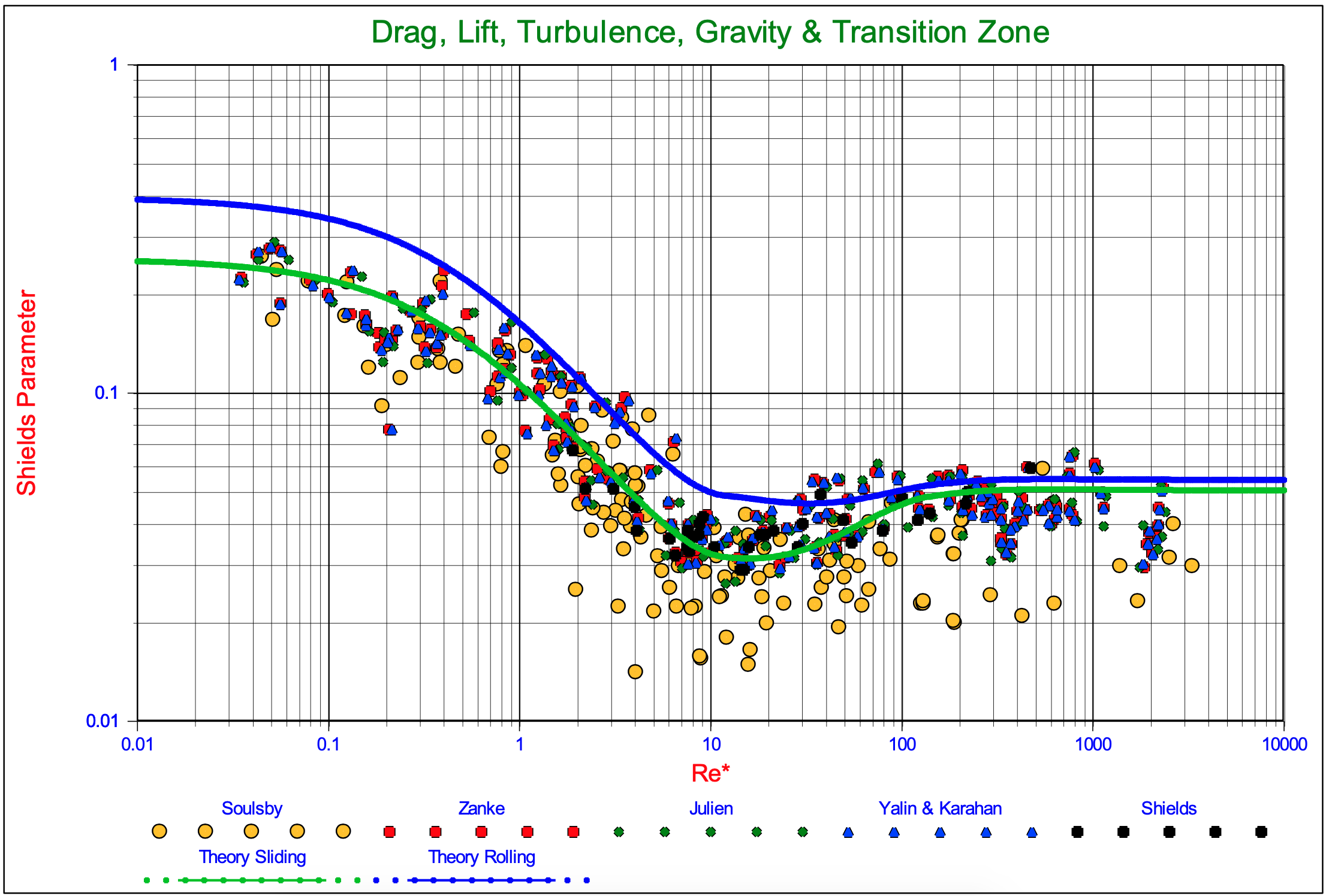
The resulting graphs are shown in Figure 5.1-15. It is clear from this figure that the Shields curve for the sliding mechanism at an exposure level of 0.5 is lower than the curve for the rolling mechanism, which leads to the main conclusion that the Shields criterion is a criterion based on bulk erosion and not on erosion of individual particles.
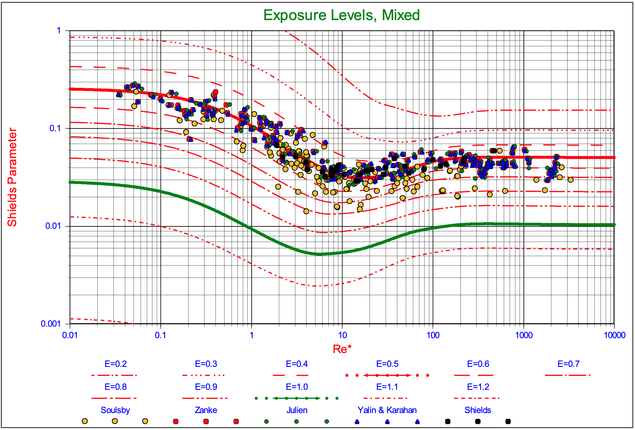
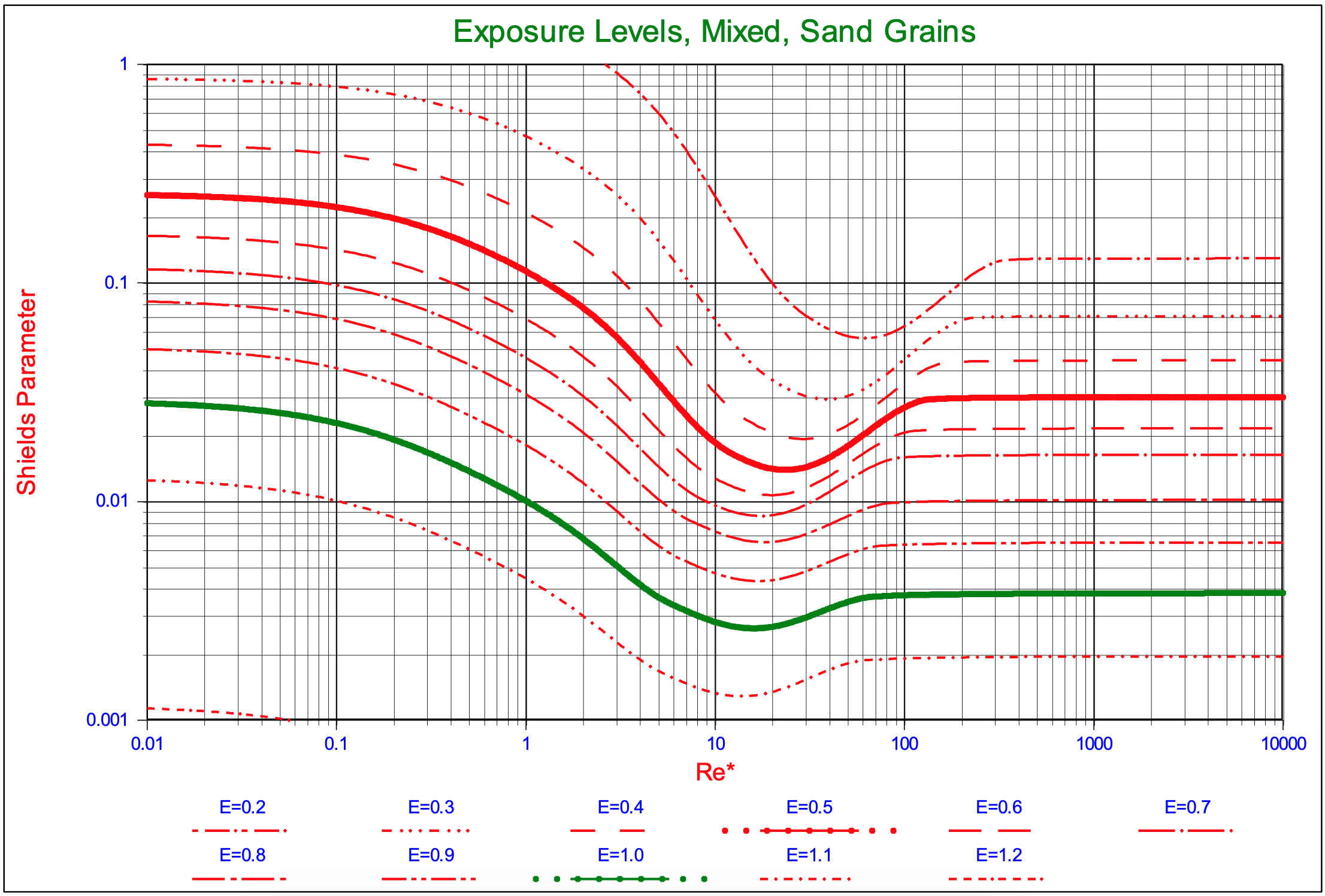
The fact that the sliding mechanism gives smaller Shields values than the rolling mechanism for an exposure level of 0.5, does not mean that this will also occur at all other exposure levels. Up to an exposure level of about 0.6 the sliding mechanism gives the smaller Shields values, while the rolling mechanism gives smaller Shields values at greater exposure levels. So the “few” particles with a very high exposure level will be subject to rolling, while the bed as a whole is subject to sliding. The lift mechanism will only occur for individual particles under experimental conditions, since the sliding or rolling mechanisms will always occur before lifting will take place. Figure 5.1-16 shows the Shields curves for different exposure levels, ranging from 0.2 to 1.2, where the curves calculated are for the sliding mechanism up to an exposure level of 0.6 and for the rolling mechanism above that.
5.1.3.10 Natural Sands and Gravels
As has been described by Miedema (2012A) and (2012B), the drag coefficient of natural sands and gravels differs from the drag coefficient of spheres. For rounded grains this difference is probably not too big, but for angular grains it is. In the laminar region at low Reynolds numbers both spheres and natural particles follow (or almost follow) the Stokes law, giving a drag coefficient of CD=24/Re, while some researchers use CD=32/Re for natural sands. In the turbulent region however the difference is much larger. At large Reynolds numbers the drag coefficient for spheres is about CD=0.445, while for natural sands and gravels values of CD=1-2 are used. Using the equation as mentioned in Julien (1995) gives Shields curves as shown in Figure 5.1-17. In the laminar region the curves are almost identical to the curves for spheres, but in the turbulent region the curves gives values of 50% to 60% of the curves for spheres, as mentioned before and as experienced by other researchers. The curves in Figure 5.1-17 are for the sliding mechanism for exposure levels up to 0.6 and the rolling mechanism for larger exposure levels.
\[\ \mathrm{C_{D}}=\frac{24}{\mathrm{R e_{D}}}+1.5\]
5.1.3.11 The Shields-Parker Diagram
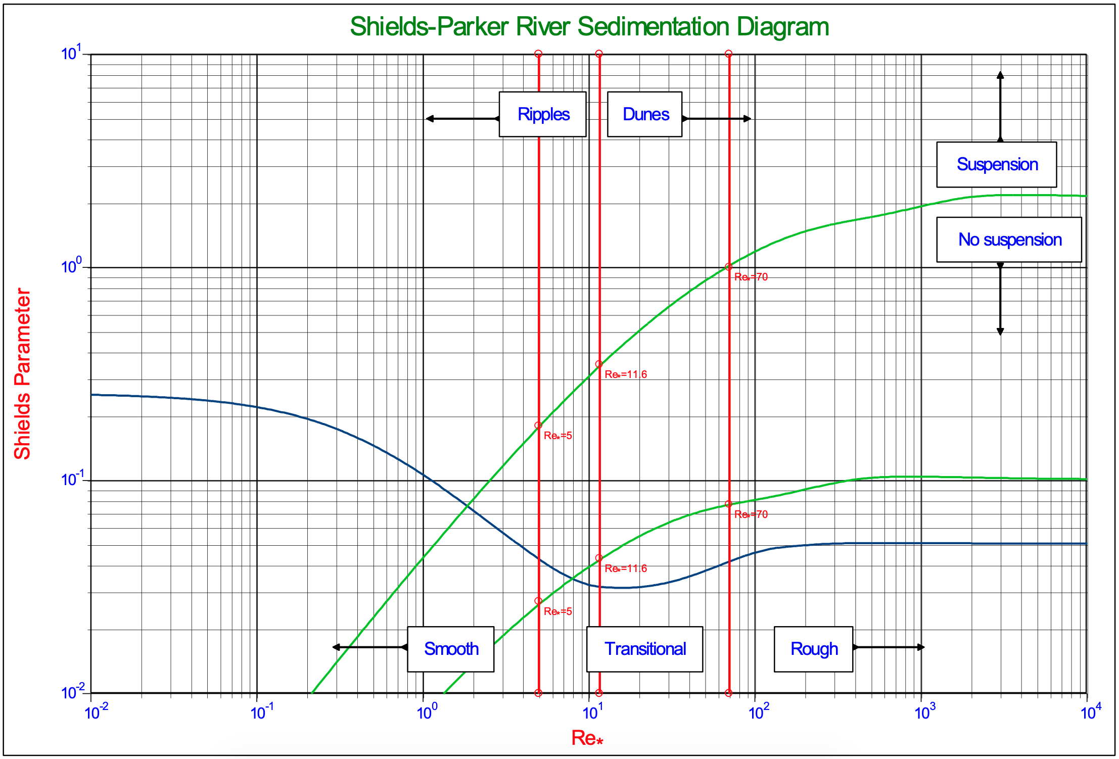
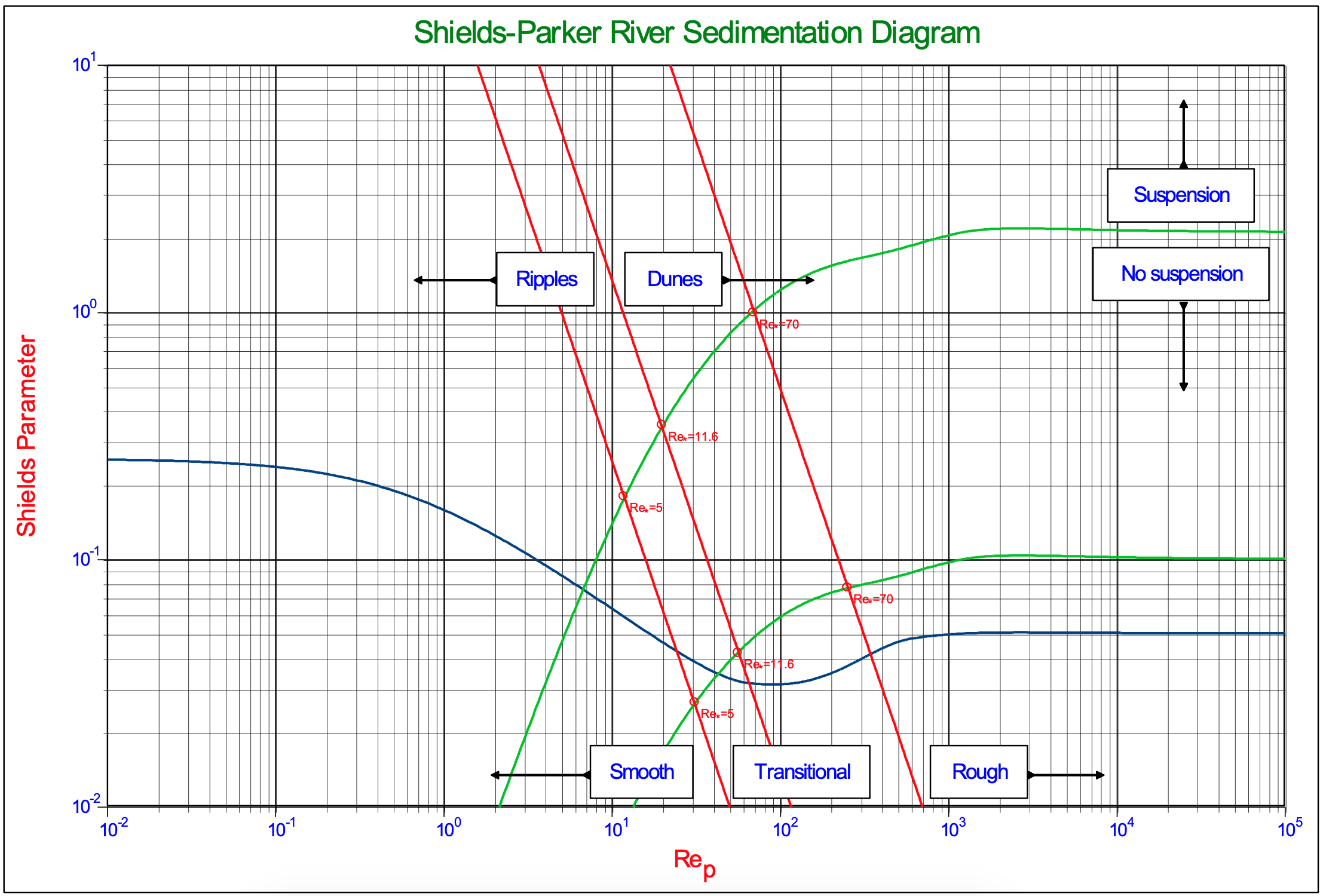
A well-known application of the Shields curve is the so called Shields-Parker diagram, showing erosion versus no erosion, suspension versus no suspension and ripples versus dunes. This diagram is shown in Figure 5.1-18 with the boundary Reynolds number on the abscissa and Figure 5.1-19 with the particle Reynolds number on the abscissa.
5.1.3.12 Conclusions & Discussion
A model to explain the Shields curve has been developed, based on realistic values of the properties involved. The model correlates well with the original data of Shields (1936), the data collected by Yalin & Karahan (1979) and the data of others. Sliding, rolling and lifting are considered as the mechanism for entrainment, where sliding correlated the best with the data. Rolling gives higher values than sliding for the Shields parameter, while pure lift only occurs in the turbulent region at even higher values of the Shields parameter than rolling. Since sliding correlates the best and the fact that the original Shields data match critical to general transport, meaning that many particles at many locations are entrained, the main mechanism is sliding. Rolling and lifting are much more mechanisms of individual particles, while sliding may mobilize the whole top layer of the particles. Rolling by pivoting can only occur if a pivot point exists, but when most particles in the top layer start to move, there often is no next particle, creating a pivot point. It can be expected however that particles having a higher exposure level than the 0.5 considered, will start to roll at lower values of the Shields parameter then predicted with the model.
Some new concepts have been introduced, comparing the model developed with already existing models. First of all the definition of the exposure and protrusion level in relation with the flow field and the use of the acting velocity and lever arm. The acting velocity and lever arm are not estimated, but determined based on taking the square root of the surface averaged square of the velocity integrated over the cross section of the particle exposed to the flow. It is surprising that previous researchers choose an average velocity or surface averaged velocity, since we are dealing with forces. To find the acting point of a stress or pressure, the stress or pressure has to be integrated over the cross section exposed to the flow in order to determine the acting point and the effective value.
The introduction of the influence of turbulence is not new, but the introduction of the effective turbulence influence, based on the factor of simultaneous occurrence is. Also here, it is not about a velocity distribution or turbulence intensity distribution, but it is about the probability of the resulting force on a particle taking into account the phase cancellations of the small eddies. The original turbulence intensity profile as proposed by Nezu & Nakagawa (1993) has been modified slightly, so not only the turbulence intensity at the virtual bed is zero, but also the derivative with respect to the distance to the wall. The laminar region is dominated by drag and small eddy turbulence, while the turbulent region is dominated by drag and lift. A transition zone is chosen for non- dimensional particle exposure heights from 5 to 70 and a sophisticated interpolation method is used.
Finally, the virtual bed level is chosen at 0.2·d below to top of the bed. In literature different values are used for the virtual bed level. Van Rijn (1984) and later Dey (1999) for example used 0.25·d. To interpret the value of the virtual bed level we have to consider that it is a value used to justify the velocity profile above the bed. Most probably, the velocity profile between the top of the grains will not follow the theoretical velocity profile, but most probably there will already be velocity at lower levels than the assumed virtual bed level. This implies that at very low exposure levels, resulting in negative protrusion levels, the velocity distribution should be corrected with respect to the theoretical profile. This also implies that the virtual bed levels for the time averaged velocities and the turbulence intensity do not necessarily have to be the same, justifying the modified turbulence intensity, but also the assumptions made by Zanke (2003). The fact that the model developed correlates very well with the data for very common values for the different properties, including the virtual bed level, proves that the model gives a good description of reality, without having the presumption of being reality.
5.1.4 Nomenclature Initiation of Motion of Particles
|
CD |
Drag coefficient |
- |
|
CL |
Lift coefficient |
- |
|
d |
Sphere, particle or grain diameter |
m |
|
D* |
The Bonneville parameter or non-dimensional grain diameter |
- |
|
E |
Exposure level |
- |
|
fD,fDrag |
Fraction of cross section exposed to drag |
- |
|
fL,fLift |
Fraction of top surface exposed to lift |
- |
|
FD |
Drag force |
N |
|
FL |
Lift force |
N |
|
FW |
Weight of a particle |
N |
|
g |
Gravitational constant |
9.81 m/s2 |
|
h |
Thickness of the layer of water |
m |
|
ks |
Roughness often chosen equal to the particle diameter |
m |
|
ks+ |
The non-dimensional roughness or roughness Reynolds number |
- |
| \(\ \boldsymbol{\ell}\) |
The point of action of the drag force |
- |
| \(\ {\ell}\) |
Mixing length |
m |
| \(\ \ell_{\text {Drag }}\) |
Drag point of action |
- |
| \(\ \ell_{\text {Lift }}\) |
Lift point of action |
- |
| \(\ \ell_{\text {Lever-D }}\) |
Additional lever arm for drag |
- |
| \(\ \ell_{\text {Lever-L }}\) |
Additional lever arm for lift |
- |
|
n |
Turbulence intensity factor |
- |
|
R |
Radius of sphere, particle or grain |
m |
|
Rsd |
The relative submerged specific density |
- |
|
ReD |
The particle drag Reynolds number |
- |
|
Re* |
Boundary Reynolds number |
- |
|
u |
Time and surface averaged velocity |
m/s |
|
u* |
Friction velocity |
m/s |
|
u+ |
Non dimensional time and surface averaged velocity |
- |
|
ur.m.s. |
Turbulence intensity |
m/s |
|
u'r.m.s. |
Modified turbulence intensity |
m/s |
|
u'n,r.m.s. |
The nth moment of the modified turbulence intensity |
m/s |
|
ueff. |
The effective modified turbulence intensity |
m/s |
|
ur.m.s.+ |
Non dimensional turbulence intensity |
- |
|
utotal+ |
Non dimensional total velocity |
- |
|
Uc |
Threshold velocity Hjulstrom |
m/s |
|
Ud |
Deposition velocity Hjulstrom |
m/s |
|
y |
Distance to the wall or virtual bed level |
m |
|
y0 |
Integration constant |
m |
|
y+ |
Non dimensional distance to the wall (Reynolds number) |
- |
|
α |
The velocity factor at a certain exposure level |
- |
|
δv |
Thickness of the viscous sub layer |
m |
|
δv+ |
The non-dimensional thickness of the viscous sub layer |
11.6 |
|
κ |
Von Karman constant |
0.412 |
|
ρl |
Liquid density |
kg/m3 |
|
ρs, ρq |
Solids density, quarts density |
kg/m3 |
|
\(\ \varphi, \phi\) |
Internal friction angle/angle of repose |
° |
| \(\ \phi_{0}\) |
The Coulomb friction angle quarts-quarts |
° |
| \(\ \phi_\text{Roll}\) |
Friction angle for rolling resistance |
° |
|
ψ |
The dilatation angle |
° |
| ψ |
The pivot angle |
° |
|
\(\ \theta\) |
The Shields parameter or non-dimensional shear stress |
- |
| \(\ \theta_{\text {sliding }}\) |
The Shields parameter for sliding |
- |
| \(\ \theta_{\text {rolling }}\) |
The Shields parameter for rolling |
- |
| \(\ \theta_{\text {lifting }}\) |
The Shields parameter for lifting |
- |
| \(\ \boldsymbol{\tau}\) |
Total shear stress |
Pa |
| \(\ \boldsymbol{\tau}_{\mathrm{t}}\) |
Turbulent shear stress |
Pa |
| \(\ \boldsymbol{\tau}_{\mathrm{v}}\) |
Viscous shear stress |
Pa |
| \(\ \boldsymbol{\tau}_{\mathrm{b}}\) |
Bed shear stress |
Pa |
| \(\ v_{\mathrm{l}}\) |
Kinematic viscosity liquid |
m2/sec |
|
μsf |
Friction coefficient usually the tangent of the internal friction angle |
- |
|
μrf |
Equivalent friction coefficient for rolling |
- |


