
5.3: Erosion, Bed Load and Suspended Load
- Page ID
- 29208

\( \newcommand{\vecs}[1]{\overset { \scriptstyle \rightharpoonup} {\mathbf{#1}} } \)
\( \newcommand{\vecd}[1]{\overset{-\!-\!\rightharpoonup}{\vphantom{a}\smash {#1}}} \)
\( \newcommand{\id}{\mathrm{id}}\) \( \newcommand{\Span}{\mathrm{span}}\)
( \newcommand{\kernel}{\mathrm{null}\,}\) \( \newcommand{\range}{\mathrm{range}\,}\)
\( \newcommand{\RealPart}{\mathrm{Re}}\) \( \newcommand{\ImaginaryPart}{\mathrm{Im}}\)
\( \newcommand{\Argument}{\mathrm{Arg}}\) \( \newcommand{\norm}[1]{\| #1 \|}\)
\( \newcommand{\inner}[2]{\langle #1, #2 \rangle}\)
\( \newcommand{\Span}{\mathrm{span}}\)
\( \newcommand{\id}{\mathrm{id}}\)
\( \newcommand{\Span}{\mathrm{span}}\)
\( \newcommand{\kernel}{\mathrm{null}\,}\)
\( \newcommand{\range}{\mathrm{range}\,}\)
\( \newcommand{\RealPart}{\mathrm{Re}}\)
\( \newcommand{\ImaginaryPart}{\mathrm{Im}}\)
\( \newcommand{\Argument}{\mathrm{Arg}}\)
\( \newcommand{\norm}[1]{\| #1 \|}\)
\( \newcommand{\inner}[2]{\langle #1, #2 \rangle}\)
\( \newcommand{\Span}{\mathrm{span}}\) \( \newcommand{\AA}{\unicode[.8,0]{x212B}}\)
\( \newcommand{\vectorA}[1]{\vec{#1}} % arrow\)
\( \newcommand{\vectorAt}[1]{\vec{\text{#1}}} % arrow\)
\( \newcommand{\vectorB}[1]{\overset { \scriptstyle \rightharpoonup} {\mathbf{#1}} } \)
\( \newcommand{\vectorC}[1]{\textbf{#1}} \)
\( \newcommand{\vectorD}[1]{\overrightarrow{#1}} \)
\( \newcommand{\vectorDt}[1]{\overrightarrow{\text{#1}}} \)
\( \newcommand{\vectE}[1]{\overset{-\!-\!\rightharpoonup}{\vphantom{a}\smash{\mathbf {#1}}}} \)
\( \newcommand{\vecs}[1]{\overset { \scriptstyle \rightharpoonup} {\mathbf{#1}} } \)
\( \newcommand{\vecd}[1]{\overset{-\!-\!\rightharpoonup}{\vphantom{a}\smash {#1}}} \)
\(\newcommand{\avec}{\mathbf a}\) \(\newcommand{\bvec}{\mathbf b}\) \(\newcommand{\cvec}{\mathbf c}\) \(\newcommand{\dvec}{\mathbf d}\) \(\newcommand{\dtil}{\widetilde{\mathbf d}}\) \(\newcommand{\evec}{\mathbf e}\) \(\newcommand{\fvec}{\mathbf f}\) \(\newcommand{\nvec}{\mathbf n}\) \(\newcommand{\pvec}{\mathbf p}\) \(\newcommand{\qvec}{\mathbf q}\) \(\newcommand{\svec}{\mathbf s}\) \(\newcommand{\tvec}{\mathbf t}\) \(\newcommand{\uvec}{\mathbf u}\) \(\newcommand{\vvec}{\mathbf v}\) \(\newcommand{\wvec}{\mathbf w}\) \(\newcommand{\xvec}{\mathbf x}\) \(\newcommand{\yvec}{\mathbf y}\) \(\newcommand{\zvec}{\mathbf z}\) \(\newcommand{\rvec}{\mathbf r}\) \(\newcommand{\mvec}{\mathbf m}\) \(\newcommand{\zerovec}{\mathbf 0}\) \(\newcommand{\onevec}{\mathbf 1}\) \(\newcommand{\real}{\mathbb R}\) \(\newcommand{\twovec}[2]{\left[\begin{array}{r}#1 \\ #2 \end{array}\right]}\) \(\newcommand{\ctwovec}[2]{\left[\begin{array}{c}#1 \\ #2 \end{array}\right]}\) \(\newcommand{\threevec}[3]{\left[\begin{array}{r}#1 \\ #2 \\ #3 \end{array}\right]}\) \(\newcommand{\cthreevec}[3]{\left[\begin{array}{c}#1 \\ #2 \\ #3 \end{array}\right]}\) \(\newcommand{\fourvec}[4]{\left[\begin{array}{r}#1 \\ #2 \\ #3 \\ #4 \end{array}\right]}\) \(\newcommand{\cfourvec}[4]{\left[\begin{array}{c}#1 \\ #2 \\ #3 \\ #4 \end{array}\right]}\) \(\newcommand{\fivevec}[5]{\left[\begin{array}{r}#1 \\ #2 \\ #3 \\ #4 \\ #5 \\ \end{array}\right]}\) \(\newcommand{\cfivevec}[5]{\left[\begin{array}{c}#1 \\ #2 \\ #3 \\ #4 \\ #5 \\ \end{array}\right]}\) \(\newcommand{\mattwo}[4]{\left[\begin{array}{rr}#1 \amp #2 \\ #3 \amp #4 \\ \end{array}\right]}\) \(\newcommand{\laspan}[1]{\text{Span}\{#1\}}\) \(\newcommand{\bcal}{\cal B}\) \(\newcommand{\ccal}{\cal C}\) \(\newcommand{\scal}{\cal S}\) \(\newcommand{\wcal}{\cal W}\) \(\newcommand{\ecal}{\cal E}\) \(\newcommand{\coords}[2]{\left\{#1\right\}_{#2}}\) \(\newcommand{\gray}[1]{\color{gray}{#1}}\) \(\newcommand{\lgray}[1]{\color{lightgray}{#1}}\) \(\newcommand{\rank}{\operatorname{rank}}\) \(\newcommand{\row}{\text{Row}}\) \(\newcommand{\col}{\text{Col}}\) \(\renewcommand{\row}{\text{Row}}\) \(\newcommand{\nul}{\text{Nul}}\) \(\newcommand{\var}{\text{Var}}\) \(\newcommand{\corr}{\text{corr}}\) \(\newcommand{\len}[1]{\left|#1\right|}\) \(\newcommand{\bbar}{\overline{\bvec}}\) \(\newcommand{\bhat}{\widehat{\bvec}}\) \(\newcommand{\bperp}{\bvec^\perp}\) \(\newcommand{\xhat}{\widehat{\xvec}}\) \(\newcommand{\vhat}{\widehat{\vvec}}\) \(\newcommand{\uhat}{\widehat{\uvec}}\) \(\newcommand{\what}{\widehat{\wvec}}\) \(\newcommand{\Sighat}{\widehat{\Sigma}}\) \(\newcommand{\lt}{<}\) \(\newcommand{\gt}{>}\) \(\newcommand{\amp}{&}\) \(\definecolor{fillinmathshade}{gray}{0.9}\)5.3.1 Introduction
The initiation of motion deals with the start of movement of particles and may be considered a lower limit for the occurrence of erosion or sediment transport. This is important for the stationary bed regime in slurry transport in order to determine at which line speed erosion will start. Under operational conditions in dredging however the line speeds are much higher resulting in a sliding bed with sheet flow or even heterogeneous flow or homogeneous flow. Models dealing with this are the 2 layer models and the 3 layer models, assuming either a sheet flow layer on top of the bed or a certain velocity and concentration distribution above the bed due to suspended load. To understand these models it is necessary to understand the basics of bed load transport and suspended load and velocity and concentration distributions.
5.3.2 Bed Load Transport in a Sheet Flow Layer
Of course there are many bed load transport equations. The Meyer-Peter Muller ( MPM) equation however is used in some of the 2 layer and 3 layer models and has the advantage of having an almost fundamental derivation as given here, reason to discuss the MPM equation.
The total sediment transport of bed load Qs can be determined by integrating the volumetric concentration Cvs(z) times the velocity U(z) over the height of the flow layer H with a bed width w.
\[\ \mathrm{Q}_{\mathrm{s}}=\mathrm{w} \cdot \int_{\mathrm{z}=\mathrm{0}}^{\mathrm{z}=\mathrm{H}} \mathrm{C}_{\mathrm{v} \mathrm{s}}(\mathrm{z}) \cdot \mathrm{U}(\mathrm{z}) \cdot \mathrm{d} \mathrm{z}\]
Bed load transport qb is often expressed in the dimensionless form:
\[\ \Phi_{\mathrm{b}}=\frac{\mathrm{q}_{\mathrm{b}}}{\mathrm{d} \cdot \sqrt{\mathrm{R}_{\mathrm{sd}} \cdot \mathrm{g} \cdot \mathrm{d}}}=\frac{\mathrm{Q}_{\mathrm{s}}}{\mathrm{d} \cdot \sqrt{\mathrm{R}_{\mathrm{sd}} \cdot \mathrm{g} \cdot \mathrm{d}} \cdot \mathrm{w}}\]
The bed load transport parameter qb is the solids flux per unit width of the bed w. The most famous bed load transport equation is the Meyer-Peter Muller (1948) equation, resulting from the fitting of a large amount of experimental data.
The original MPM equation includes the critical Shields parameter, giving:
\[\ \Phi_{\mathrm{b}}=\frac{\mathrm{Q}_{\mathrm{s}}}{\mathrm{d} \cdot \sqrt{\mathrm{R}_{\mathrm{s} \mathrm{d}} \cdot \mathrm{g} \cdot \mathrm{d}} \cdot \mathrm{w}}=\mathrm{\alpha} \cdot\left(\begin{array}{lllll}\theta-\theta_{\mathrm{c r}} \end{array}\right)^{\boldsymbol{\beta}} \quad\text{ with: }\quad \boldsymbol{\alpha}=\mathrm{8} \quad\text{ and }\quad \boldsymbol{\beta}=\mathrm{1 . 5}\]
The Shields parameter, the dimensionless bed shear stress, is defined as:
\[\ \theta=\frac{\tau_{\mathrm{b}}}{\rho_{\mathrm{l}} \cdot \mathrm{R}_{\mathrm{sd}} \cdot \mathrm{g} \cdot \mathrm{d}}=\frac{\mathrm{u}_{*}^{2}}{\mathrm{R}_{\mathrm{sd}} \cdot \mathrm{g} \cdot \mathrm{d}} \quad$ or $\quad \mathrm{u}_{*}=\sqrt{\theta \cdot \mathrm{R}_{\mathrm{sd}} \cdot \mathrm{g} \cdot \mathrm{d}}\]
The MPM equation can almost be derived from the velocity and concentration distribution in a sheet flow layer above the bed, assuming a stationary bed. Pugh & Wilson (1999) found a relation for the velocity at the top of the sheet flow layer with a stationary bed. This relation is modified here for a sliding bed, giving:
\[\ \mathrm{U}_{\mathrm{H}}=\gamma \cdot \mathrm{u}_{*}=\gamma \cdot \sqrt{\frac{\lambda_{\mathrm{b}}}{\mathrm{8}}} \cdot \mathrm{U}_{\text {mean }} \quad\text{ with: }\quad \gamma=9.4\]
The shear stress on the sheet flow layer has to be transferred to the bed by sliding friction. It is assumed that this sliding friction is related to the internal friction angle, giving for the thickness of the sheet flow layer:
\[\ \mathrm{H}=\frac{\tau_{\mathrm{b}}}{\rho_{\mathrm{l}} \cdot \mathrm{R}_{\mathrm{s} \mathrm{d}} \cdot \mathrm{g} \cdot \mathrm{C}_{\mathrm{v} \mathrm{s}, \mathrm{s} \mathrm{f}} \cdot \tan (\varphi)} \approx \frac{\mathrm{2} \cdot \mathrm{\theta} \cdot \mathrm{d}}{\mathrm{C}_{\mathrm{v} \mathrm{b}} \cdot \tan (\varphi)}
\quad\text{ With: }\quad \mathrm{C}_{\mathrm{v} \mathrm{s}, \mathrm{s} \mathrm{f}} \approx \mathrm{0} . \mathrm{5} \cdot \mathrm{C}_{\mathrm{v} \mathrm{b}} \quad\text{ and }\quad \tan (\varphi)=\mathrm{0 . 5 7 7}\]
Assuming a linear concentration distribution in the sheet flow layer, starting at the bed concentration Cvb at the bottom of the sheet flow layer and ending with a concentration of zero at the top of the sheet flow layer gives:
\[\ \mathrm{C}_{\mathrm{v s}}(\mathrm{z})=\mathrm{C}_{\mathrm{v} \mathrm{b}} \cdot\left(\frac{\mathrm{H}-\mathrm{z}}{\mathrm{H}}\right)\]
With z the vertical coordinate starting at the bottom of the sheet flow layer and increasing going upwards. The velocity in the sheet flow layer is assumed to start with zero at the bottom and ends with UH at the top following a power law according to:
\[\ \mathrm{U}(\mathrm{z})=\mathrm{U}_{\mathrm{H}} \cdot\left(\frac{\mathrm{z}}{\mathrm{H}}\right)^{\mathrm{n}}\]
The transport of solids in the sheet flow layer can now be determined by integration of the spatial concentration profile times the velocity profile in the sheet flow layer:
\[\ \begin{array}\mathrm{Q}_{\mathrm{s}}&=\mathrm{w} \cdot \int_{\mathrm{0}}^{\mathrm{H}} \mathrm{C}_{\mathrm{v} \mathrm{s}}(\mathrm{z}) \cdot \mathrm{U}(\mathrm{z}) \cdot \mathrm{d} \mathrm{z}=\mathrm{w} \cdot \int_{\mathrm{0}}^{\mathrm{H}} \mathrm{C}_{\mathrm{v} \mathrm{b}} \cdot\left(\frac{\mathrm{H}-\mathrm{z}}{\mathrm{H}}\right) \cdot \mathrm{U}_{\mathrm{H}} \cdot\left(\frac{\mathrm{z}}{\mathrm{H}}\right)^{\mathrm{n}} \cdot \mathrm{d} \mathrm{z} \\
\mathrm{Q}_{\mathrm{s}}&=\mathrm{w} \cdot \mathrm{C}_{\mathrm{v} \mathrm{b}} \cdot \mathrm{U}_{\mathrm{H}} \cdot \int_{\mathrm{0}}^{\mathrm{H}}\left(\frac{\mathrm{H}-\mathrm{z}}{\mathrm{H}}\right) \cdot\left(\frac{\mathrm{z}}{\mathrm{H}}\right)^{\mathrm{n}} \cdot \mathrm{d} \mathrm{z}\end{array}\]
This can be rewritten to:
\[\ \mathrm{Q}_{\mathrm{s}}=\mathrm{w} \cdot \mathrm{C}_{\mathrm{v} \mathrm{b}} \cdot \mathrm{U}_{\mathrm{H}} \cdot \int_{\mathrm{0}}^{\mathrm{H}}\left(\left(\frac{\mathrm{z}}{\mathrm{H}}\right)^{\mathrm{n}}-\left(\frac{\mathrm{z}}{\mathrm{H}}\right)^{\mathrm{n}+1}\right) \mathrm{d} \mathrm{z}\]
Integration gives:
\[\ \mathrm{Q}_{\mathrm{s}}=\mathrm{w} \cdot \mathrm{C}_{\mathrm{v} \mathrm{b}} \cdot \mathrm{U}_{\mathrm{H}} \cdot \mathrm{H} \cdot\left(\frac{\mathrm{1}}{(\mathrm{n}+\mathrm{1})} \cdot\left(\frac{\mathrm{z}}{\mathrm{H}}\right)^{\mathrm{n}+1}-\frac{\mathrm{1}}{(\mathrm{n}+\mathrm{2})} \cdot\left(\frac{\mathrm{z}}{\mathrm{H}}\right)^{\mathrm{n}+2}\right)_{0}^{\mathrm{H}}\]
With integration from zero to the thickness of the sheet flow layer this gives:
\[\ \mathrm{Q_{s}=w \cdot C_{\mathrm{v b}} \cdot U_{H} \cdot H \cdot\left(\frac{1}{(n+1) \cdot(n+2)}\right)}\]
Substitution of the velocity at the top of the sheet flow layer and the thickness of the sheet flow layer gives:
\[\ \begin{array} \begin{array}\mathrm{Q}_{\mathrm{s}}&=\mathrm{w} \cdot \mathrm{C}_{\mathrm{v} \mathrm{b}} \cdot \gamma \cdot \sqrt{\mathrm{\theta} \cdot \mathrm{R}_{\mathrm{sd}} \cdot \mathrm{g} \cdot \mathrm{d}} \cdot \frac{\mathrm{2} \cdot \mathrm{\theta} \cdot \mathrm{d}}{\mathrm{C}_{\mathrm{v} \mathrm{b}} \cdot \tan (\varphi)} \cdot\left(\frac{\mathrm{1}}{(\mathrm{n}+\mathrm{1}) \cdot(\mathrm{n}+\mathrm{2})}\right)\\
\mathrm{Q}_{\mathrm{s}}&=\frac{\mathrm{2} \cdot \boldsymbol{\gamma}}{(\mathrm{n}+\mathrm{1}) \cdot(\mathrm{n}+\mathrm{2}) \cdot \tan (\varphi)} \cdot(\mathrm{w} \cdot \mathrm{d} \cdot \sqrt{\mathrm{R}_{\mathrm{s}} \mathrm{d} \cdot \mathrm{g} \cdot \mathrm{d}}) \cdot \mathrm{\theta}^{3 / 2}\end{array}\]
So the dimensionless bed load transport parameter is:
\[\ \Phi_{\mathrm{b}}=\frac{Q_{\mathrm{s}}}{\mathrm{w} \cdot \mathrm{d} \cdot \sqrt{\mathrm{R}_{\mathrm{sd}} \cdot \mathrm{g} \cdot \mathrm{d}}}=\frac{\mathrm{2} \cdot \gamma}{(\mathrm{n}+\mathrm{1}) \cdot(\mathrm{n}+\mathrm{2}) \cdot \tan (\varphi)} \cdot \theta^{\mathrm{3} / 2}\]
This is almost equal to the MPM equation, except for the critical Shields parameter θcr in the MPM equation. For medium and coarse sands the value of this critical Shields parameter lies between 0.03 and 0.05. The velocities in slurry flow are high, resulting in much higher values of the Shields parameter, so this critical Shields parameter θcr can be ignored. With an exponent n=1 for the velocity distribution, an angle of internal friction at the top of the bed giving tan(φ)=0.577 and a parameter γ=9.4 for the velocity at the top of the sheet flow layer, a factor α=5.43 is found, while the original MPM equation uses α=8. It is however questionable whether the internal friction angle of 30° at the top of the bed is correct, a smaller angle of internal friction would be expected, resulting in a higher value of α. Also the values of n=1 and γ=9.4 can be questioned. The equation found can thus easily be matched with the 3 coefficients involved.
5.3.3 Suspended Load Transport in Open Channel Flow
5.3.3.1Governing Equations
Dey (2014) gives a clear description of suspended load transport. A summary is given here. If particles are surrounded by the carrier liquid for a long period of time they are in suspension and the transport mode is named suspended load. Convection of turbulence results in exchange of mass and momentum, including the particles, between layers of liquid flow. Random motion and turbulence results in diffusion, while velocity gradients, due to bulk motion of the liquid, result in advection. When gravity, resulting in the settling of particles, is counterbalanced by turbulence induced diffusion, particles stay in suspension and are transported by the time averaged flow velocity. There is however an active interchange of particles between bed load and suspended load. Suspended load is always accompanied by bed load. The total sediment transport of suspended solids Qs can be determined by integrating the volumetric concentration Cvs(z) times the velocity U(z) over the height of the flow layer H with a bed width w in case of a 2 dimensional geometry.
\[\ \mathrm{Q}_{\mathrm{s}}=\mathrm{w} \cdot \int_{\mathrm{z}=\mathrm{0}}^{\mathrm{z}=\mathrm{H}} \mathrm{C}_{\mathrm{v} \mathrm{s}}(\mathrm{z}) \cdot \mathrm{U}(\mathrm{z}) \cdot \mathrm{d} \mathrm{z}\]
To solve this equation, both the concentration distribution and the velocity distribution have to be known. Now what is the distribution of the suspended sediment within the liquid (water) layer with height H? The generalised 3 dimensional advection-diffusion equation for a low concentration of suspended sediment motion in an incompressible liquid flow is:
\[\ \begin{array}{} \text{Part I}&: \frac{\partial \mathrm{C}}{\partial \mathrm{t}}\\
\text{Part II} &: +\overline{\mathrm{u}} \cdot \frac{\partial \mathrm{C}}{\partial \mathrm{x}}+\overline{\mathrm{v}} \cdot \frac{\partial \mathrm{C}}{\partial \mathrm{y}}+\overline{\mathrm{w}} \cdot \frac{\partial \mathrm{C}}{\partial \mathrm{z}}+\mathrm{C} \cdot\left(\frac{\partial \overline{\mathrm{u}}}{\partial \mathrm{x}}+\frac{\partial \overline{\mathrm{v}}}{\partial \mathrm{y}}+\frac{\partial \overline{\mathrm{w}}}{\partial \mathrm{z}}\right)\\
\text{Part III} &: =\dot{\mathrm{C}}\\
\text{Part IV} &: +\frac{\partial}{\partial \mathrm{x}} \cdot\left(\left(\varepsilon_{\mathrm{m}}+\varepsilon_{\mathrm{s x}}\right) \cdot \frac{\partial \mathrm{C}}{\partial \mathrm{x}}\right)+\frac{\partial}{\partial \mathrm{y}} \cdot\left(\left(\varepsilon_{\mathrm{m}}+\varepsilon_{\mathrm{s y}}\right) \cdot \frac{\partial \mathrm{C}}{\partial \mathrm{y}}\right)+\frac{\partial}{\partial \mathrm{z}} \cdot\left(\left(\varepsilon_{\mathrm{m}}+\varepsilon_{\mathrm{s} \mathrm{z}}\right) \cdot \frac{\partial \mathrm{C}}{\partial \mathrm{z}}\right)\end{array}\]
Part I is the local change of concentration due to time. Part II is the advection of concentration. Part III the rate of change of state of concentration. According to the conservation of mass, this term is the production or dissipation rate per unit volume and is equal to zero. Part IV the diffusion and the mixing of concentration. In viscous flow, the molecular diffusion is prevalent (εm≠0) and the turbulent diffusion does not exist (εsx=εsy=εsz=0). In contrast, in turbulent flow, molecular diffusion is negligible (εm≈0) in comparison to turbulent diffusion (εsx,εsy,εsz»0). In a stationary 2 dimensional situation, with z the vertical coordinate, the equation reduces to, with on the left hand side the entrainment flux and on the right hand side the depositional flux:
\[\ \overline{\mathrm{w}} \cdot \frac{\partial \mathrm{C}}{\partial \mathrm{z}}=\frac{\partial}{\partial \mathrm{z}} \cdot\left(\varepsilon_{\mathrm{s} \mathrm{z}} \cdot \frac{\partial \mathrm{C}}{\partial \mathrm{z}}\right)\]
Substituting the vertical velocity component by the terminal settling velocity (excluding hindered settling), replacing the notation of the sediment diffusivity in z-direction εsz by εs and integrating the equation, gives:
\[\ \mathrm{v}_{\mathrm{t}} \cdot \mathrm{C}+\varepsilon_{\mathrm{s}} \cdot \frac{\partial \mathrm{C}}{\partial \mathrm{z}}=\mathrm{0}\]
Now in a stationary situation, the mean vertical velocity of the particles is zero. One can say however that a fraction of the particles is subjected to the downwards movement by settling, while the remaining fraction is moving upwards by diffusion. This would mean that the concentration in the first term has to be multiplied by a factor smaller than 1. Most probably this factor depends on the particle size, but also on the local concentration. One can also compensate for this by choosing an empirical equation for the diffusivity.
5.3.3.2A Physical Explanation
Particles settle through gravity downwards towards the bed with a terminal settling velocity vt. As the particles settle, a concentration gradient develops, with an increasing concentration downwards. Turbulence however results in an upwards flux of solids maintaining suspended sediment transport. In an equilibrium situation, there is a balance between the downwards settling motion and the upwards diffusion of particles. In a stationary situation it is possible to describe this mathematically.
The downwards flux of solids per unit area of a plane parallel to the bed is (including hindered settling):
\[\ \mathrm{q}_{\mathrm{s}, \text { down }}(\mathrm{z})=\mathrm{C}_{\mathrm{v s}}(\mathrm{z}) \cdot \mathrm{v}_{\mathrm{t}} \cdot\left(\mathrm{1}-\mathrm{C}_{\mathrm{v s}}(\mathrm{z})\right)^{\boldsymbol{\beta}}\]
The exchange of eddies between layers in the turbulent flow results in a flux of solids between these layers, by random turbulent interactions between layers giving mixing at all levels and therefore a transport from areas with a high concentration into areas with a low concentration. This upwards flux of solids per unit area parallel to the bed is:
\[\ \mathrm{q}_{\mathrm{s}, \mathrm{u p}}(\mathrm{z})=-\varepsilon_{\mathrm{s}} \cdot \frac{\mathrm{d} \mathrm{C}_{\mathrm{v} \mathrm{s}}(\mathrm{z})}{\mathrm{d} \mathrm{z}}\]
The negative sign results from the fact that the sediment flux is upwards, while the concentration gradient is positive downwards. The sediment exchange by turbulence is a diffusion process. This gives for an equilibrium situation:
\[\ \begin{array}{left} \mathrm{q}_{\mathrm{s}, \mathrm{u} \mathrm{p}}(\mathrm{z})=\mathrm{q}_{\mathrm{s}, \operatorname{down}}(\mathrm{z})\\
-\varepsilon_{\mathrm{s}} \cdot \frac{\mathrm{d} \mathrm{C}_{\mathrm{v s}}(\mathrm{z})}{\mathrm{d} \mathrm{z}}=\mathrm{C}_{\mathrm{v s}}(\mathrm{z}) \cdot \mathrm{v}_{\mathrm{t}} \cdot\left(\mathrm{1}-\mathrm{C}_{\mathrm{v} \mathrm{s}}(\mathrm{z})\right)^{\beta}\\
\mathrm{C}_{\mathrm{v s}}(\mathrm{z}) \cdot \mathrm{v}_{\mathrm{t}} \cdot\left(\mathrm{1}-\mathrm{C}_{\mathrm{v} \mathrm{s}}(\mathrm{z})\right)^{\beta}+\varepsilon_{\mathrm{s}} \cdot \frac{\mathrm{d} \mathrm{C}_{\mathrm{v} \mathrm{s}}(\mathrm{z})}{\mathrm{d} \mathrm{z}}=\mathrm{0}\end{array}\]
For the shear stress based on the eddy diffusivity εm we can write:
\[\ \tau(\mathrm{z})=\rho_{\mathrm{l}} \cdot \varepsilon_{\mathrm{m}} \cdot \frac{\mathrm{d U}(\mathrm{z})}{\mathrm{d} \mathrm{z}}\]
The sediment mass diffusivity εs is almost equal to the liquid eddy momentum diffusivity εm for small particles. For larger particles βsm is smaller than 1.
\[\ \varepsilon_{\mathrm{s}} \approx \beta_{\mathrm{sm}} \cdot \varepsilon_{\mathrm{m}}\]
With: εm=κ·u*·f(z) the eddy diffusivity. The models solving this problem found in literature are all for open channel flow. It is the questing whether these solutions are suitable for pipe flow. It is also possible that models not suitable for open channel flow, are suitable for pipe flow. Reason to discuss a number of basic models.
5.3.3.3 Law of the Wall Approach (Rouse (1937))
In the turbulent layer the total shear stress contains only the turbulent shear stress. Integration gives the famous logarithmic velocity profile (Law of the Wall):
\[\ \mathrm{U ( z )}=\frac{\mathrm{u}_{*}}{\mathrm{\kappa}} \cdot \ln \left(\frac{\mathrm{z}}{\mathrm{z}_{\mathrm{0}}}\right)\]
This gives for the velocity gradient:
\[\ \frac{\mathrm{d} \mathrm{U}(\mathrm{z})}{\mathrm{d z}}=\frac{\mathrm{u}_{*}}{\mathrm{\kappa} \cdot \mathrm{z}}\]
The definition of the friction velocity u* gives:
\[\ \mathrm{u}_{*}=\sqrt{\frac{\tau_{\mathrm{b}}}{\rho_{\mathrm{l}}}} \Rightarrow \frac{\tau_{\mathrm{b}}}{\rho_{\mathrm{l}}}=\mathrm{u}_{*}^{\mathrm{2}}\]
Now we can write for the ratio shear stress to liquid density:
\[\ \frac{\tau(\mathrm{z})}{\rho_{\mathrm{l}}}=\varepsilon_{\mathrm{m}} \cdot \frac{\mathrm{d U}(\mathrm{z})}{\mathrm{d} \mathrm{z}}=\mathrm{\kappa} \cdot \mathrm{u}_{*} \cdot \mathrm{z} \cdot \frac{\mathrm{d U}(\mathrm{z})}{\mathrm{d} \mathrm{z}}\]
Based on the Law of the Wall, a linear decrease of the shear stress resulting from eddy viscosity, starting with the bed shear stress at the bed and ending at zero at the free surface, the following can be derived:
\[\ \frac{\tau(\mathrm{z})}{\rho_{\mathrm{l}}}=\frac{\tau_{\mathrm{b}}}{\rho_{\mathrm{l}}} \cdot\left(\frac{\mathrm{H}-\mathrm{z}}{\mathrm{H}}\right)=\mathrm{u}_{*}^{\mathrm{2}} \cdot\left(\frac{\mathrm{H}-\mathrm{z}}{\mathrm{H}}\right)=\varepsilon_{\mathrm{m}} \cdot \frac{\mathrm{d} \mathrm{U}(\mathrm{z})}{\mathrm{d} \mathrm{z}}=\mathrm{\kappa} \cdot \mathrm{u}_{*} \cdot \mathrm{z} \cdot \frac{\mathrm{d} \mathrm{U}(\mathrm{z})}{\mathrm{d} \mathrm{z}}\]
This gives for the momentum diffusivity and the sediment mass diffusivity:
\[\ \varepsilon_{\mathrm{m}}=\kappa \cdot \mathrm{u}_{*} \cdot \mathrm{z} \cdot\left(\frac{\mathrm{H}-\mathrm{z}}{\mathrm{H}}\right) \quad\text{ and }\quad \varepsilon_{\mathrm{s}}=\beta_{\mathrm{sm}} \cdot \mathrm{\kappa} \cdot \mathrm{u}_{*} \cdot \mathrm{z} \cdot\left(\frac{\mathrm{H}-\mathrm{z}}{\mathrm{H}}\right)\]
This upwards flux of solids per unit area parallel to the bed is now:
\[\ \mathrm{q}_{\mathrm{s}, \mathrm{u p}}(\mathrm{z})=-\beta_{\mathrm{s m}} \cdot \mathrm{\kappa} \cdot \mathrm{u}_{*} \cdot \mathrm{z} \cdot\left(\frac{\mathrm{H}-\mathrm{z}}{\mathrm{H}}\right) \cdot \frac{\mathrm{d} \mathrm{C}_{\mathrm{v} \mathrm{s}}(\mathrm{z})}{\mathrm{d} \mathrm{z}}\]
Making the upwards flux and downwards flux of solids equal gives:
\[\ \mathrm{q}_{\mathrm{s}, \mathrm{u p}}(\mathrm{z})=\mathrm{q}_{\mathrm{s}, \text { down }}(\mathrm{z})
-\beta_{\mathrm{s m}} \cdot \mathrm{\kappa} \cdot \mathrm{u}_{*} \cdot \mathrm{z} \cdot\left(\frac{\mathrm{H}-\mathrm{z}}{\mathrm{H}}\right) \cdot \frac{\mathrm{d} \mathrm{C}_{\mathrm{v} \mathrm{s}}(\mathrm{z})}{\mathrm{d} \mathrm{z}}=\mathrm{C}_{\mathrm{v} \mathrm{s}}(\mathrm{z}) \cdot \mathrm{v}_{\mathrm{t}} \cdot\left(1-\mathrm{C}_{\mathrm{v} \mathrm{s}}(\mathrm{z})\right)^{\beta}\]
Giving the differential equation:
\[\ \mathrm{C}_{\mathrm{v s}}(\mathrm{z}) \cdot \mathrm{v}_{\mathrm{t}} \cdot\left(\mathrm{1}-\mathrm{C}_{\mathrm{v} \mathrm{s}}(\mathrm{z})\right)^{\beta}+\beta_{\mathrm{s m}} \cdot \mathrm{\kappa} \cdot \mathrm{u}_{*} \cdot \mathrm{z} \cdot\left(\frac{\mathrm{H}-\mathrm{z}}{\mathrm{H}}\right) \cdot \frac{\mathrm{d} \mathrm{C}_{\mathrm{v} \mathrm{s}}(\mathrm{z})}{\mathrm{d} \mathrm{z}}=\mathrm{0}\]
This equation can be solved assuming there is no hindered settling, reducing the differential equation to:
\[\ \mathrm{C}_{\mathrm{v s}}(\mathrm{z}) \cdot \mathrm{v}_{\mathrm{t}}+\beta_{\mathrm{s m}} \cdot \mathrm{\kappa} \cdot \mathrm{u}_{*} \cdot \mathrm{z} \cdot\left(\frac{\mathrm{H}-\mathrm{z}}{\mathrm{H}}\right) \cdot \frac{\mathrm{d} \mathrm{C}_{\mathrm{v} \mathrm{s}}(\mathrm{z})}{\mathrm{d} \mathrm{z}}=\mathrm{0}\]
Separating the variables gives:
\[\ \frac{\mathrm{d} \mathrm{C}_{\mathrm{v} \mathrm{s}}(\mathrm{z})}{\mathrm{C}_{\mathrm{v} \mathrm{s}}(\mathrm{z})}=-\left(\frac{\mathrm{v}_{\mathrm{t}}}{\beta_{\mathrm{s m}} \cdot \mathrm{\kappa} \cdot \mathrm{u}_{*}}\right) \cdot\left(\frac{\mathrm{1}}{\mathrm{z}}\right) \cdot\left(\frac{\mathrm{H}}{\mathrm{H}-\mathrm{z}}\right) \cdot \mathrm{d} \mathrm{z}\]
The solution of this differential equation is:
\[\ \ln \left(\mathrm{C}_{\mathrm{v s}}(\mathrm{z})\right)=\left(\frac{\mathrm{v}_{\mathrm{t}}}{\beta_{\mathrm{s m}} \cdot \mathrm{\kappa} \cdot \mathrm{u}_{*}}\right) \cdot \ln \left(\frac{\mathrm{z}-\mathrm{H}}{\mathrm{z}}\right)+\mathrm{C}\]
If the value of the concentration Cvs(a) is known at an elevation a above the bed, the integration constant C can be solved.
\[\ \begin{array}\ln \left(\mathrm{C}_{\mathrm{v s}}(\mathrm{a})\right)=\left(\frac{\mathrm{v}_{\mathrm{t}}}{\beta_{\mathrm{s m}} \cdot \mathrm{\kappa} \cdot \mathrm{u}_{*}}\right) \cdot \ln \left(\frac{\mathrm{a}-\mathrm{H}}{\mathrm{a}}\right)+\mathrm{C}\\
\mathrm{C}=\ln \left(\mathrm{C}_{\mathrm{v} \mathrm{s}}(\mathrm{a})\right)-\left(\frac{\mathrm{v}_{\mathrm{t}}}{\beta_{\mathrm{s m}} \cdot \mathrm{\kappa} \cdot \mathrm{u}_{*}}\right) \cdot \ln \left(\frac{\mathrm{a}-\mathrm{H}}{\mathrm{a}}\right)\\
\mathrm{C}=\ln \left(\mathrm{C}_{\mathrm{v} \mathrm{s}}(\mathrm{a})\right)+\left(\frac{\mathrm{v}_{\mathrm{t}}}{\beta_{\mathrm{s m}} \cdot \mathrm{\kappa} \cdot \mathrm{u}_{*}}\right) \cdot \ln \left(\frac{\mathrm{a}}{\mathrm{a}-\mathrm{H}}\right)\end{array}\]
This gives the Rouse (1937) profile:
\[\ \begin{array}\ln \left(\mathrm{C}_{\mathrm{v s}}(\mathrm{z})\right)&=\ln \left(\mathrm{C}_{\mathrm{v s}}(\mathrm{a})\right)+\left(\frac{\mathrm{v}_{\mathrm{t}}}{\beta_{\mathrm{s m}} \cdot \mathrm{\kappa} \cdot \mathrm{u}_{*}}\right) \cdot\left(\ln \left(\frac{\mathrm{z}-\mathrm{H}}{\mathrm{z}}\right)+\ln \left(\frac{\mathrm{a}}{\mathrm{a}-\mathrm{H}}\right)\right)\\
\ln \left(\frac{\mathrm{C}_{\mathrm{v} \mathrm{s}}(\mathrm{z})}{\mathrm{C}_{\mathrm{v} \mathrm{s}}(\mathrm{a})}\right)&=\ln \left(\left(\left(\frac{\mathrm{z}-\mathrm{H}}{\mathrm{z}}\right) \cdot\left (\frac{\mathrm{a}}{\mathrm{a}-\mathrm{H}}\right)\right)^\left(\frac{\mathrm{v}_{\mathrm{t}}}{\beta_{\mathrm{sm}} \cdot \mathrm{\kappa} \cdot \mathrm{u}_{*}}\right)\right)\\
\frac{\mathrm{C}_{\mathrm{v} \mathrm{s}}(\mathrm{z})}{\mathrm{C}_{\mathrm{v} \mathrm{s}}(\mathrm{a})}&=\left(\left(\frac{\mathrm{H}-\mathrm{z}}{\mathrm{z}}\right) \cdot\left(\frac{\mathrm{a}}{\mathrm{H}-\mathrm{a}}\right)\right)^\left(\frac{\mathrm{v}_{\mathrm{t}}}{\beta_{\mathrm{sm}} \cdot \mathrm{\kappa} \cdot \mathrm{u}_{*}}\right)\end{array}\]
The so called Rouse number is the power in this equation:
\[\ \mathrm{P}=\zeta=\left(\frac{\mathrm{v}_{\mathrm{t}}}{\beta_{\mathrm{sm}} \cdot \mathrm{\kappa} \cdot \mathrm{u}_{*}}\right) \quad\text{ with: }\quad \beta_{\mathrm{sm}} \approx \mathrm{1} \quad \Rightarrow \quad \mathrm{P}=\left(\frac{\mathrm{v}_{\mathrm{t}}}{\mathrm{\kappa} \cdot \mathrm{u}_{*}}\right)\]
The solution found results in the so called Rouse (1937) profiles for the concentration. In literature the elevation a is often chosen to be 0.05·H, since at an elevation 0 the solution would give an infinite concentration. This results from the parabolic distribution of the diffusivity as assumed by Rouse. The governing equations are derived for low concentrations, not containing hindered settling. The solution however predicts high concentrations near the bed, requiring hindered settling.
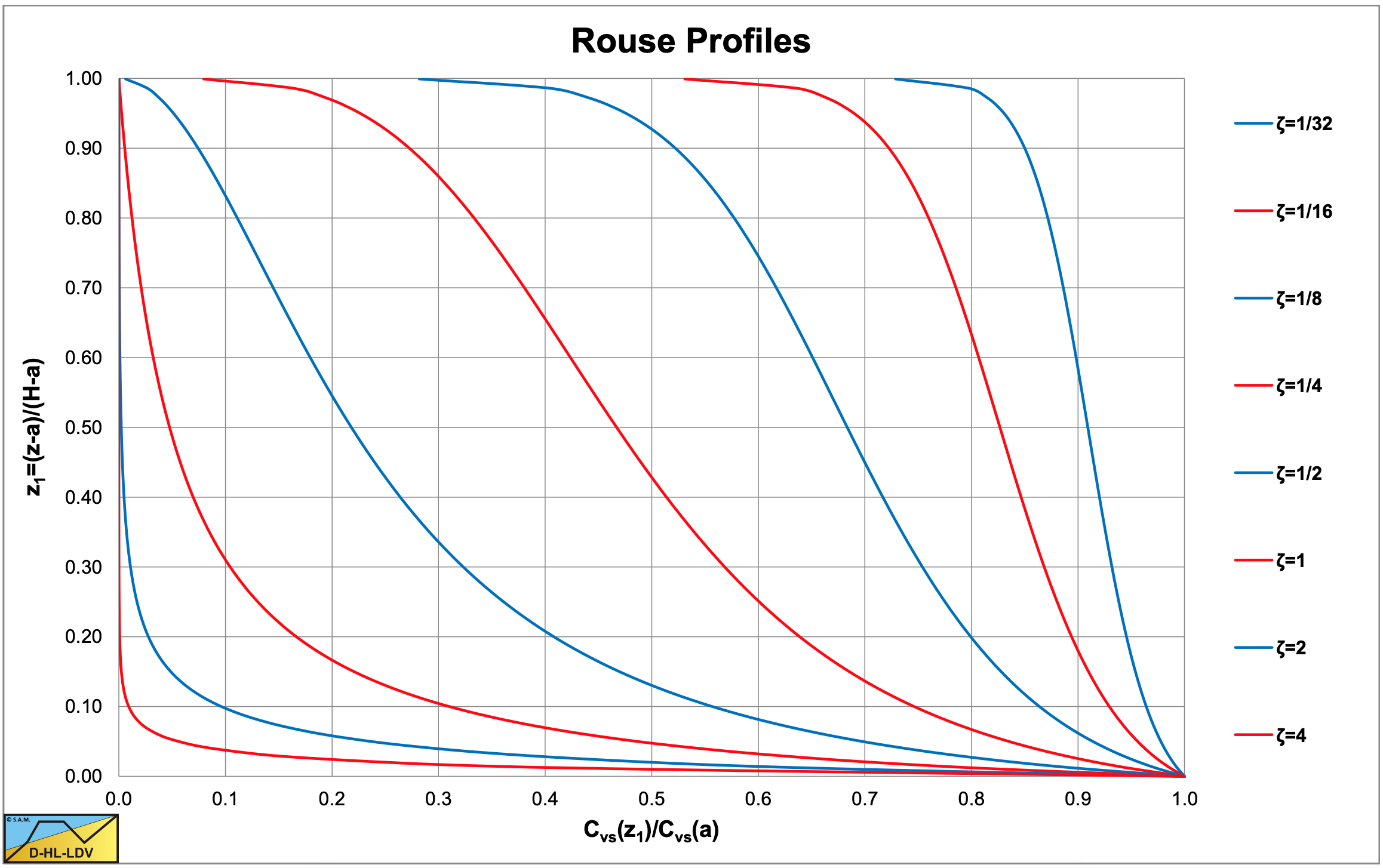
Figure 5.3-1 shows the Rouse profiles for different values of the Rouse number P or ζ, ranging from 1/32 (small particles) to 4 (large particles). The value of a is chosen a=0.05·H, the abscissa is the concentration ratio Cvs(z1)/Cvs(a) and the ordinate z1=(z-a)/(H-a). Cvs(a) is the concentration at elevation a and often considered the concentration at the bed.
5.3.3.4 The Constant Diffusivity Approach
If we assume the diffusivity is a constant, the differential equation can be solved. Giving the differential equation in the equilibrium situation:
\[\ \mathrm{C}_{\mathrm{v s}}(\mathrm{z}) \cdot \mathrm{v}_{\mathrm{t}} \cdot\left(1-\mathrm{C}_{\mathrm{v} \mathrm{s}}(\mathrm{z})\right)^{\boldsymbol{\beta}}+\boldsymbol{\beta}_{\mathrm{s m}} \cdot \boldsymbol{\varepsilon}_{\mathrm{m}} \cdot \frac{\mathrm{d} \mathrm{C}_{\mathrm{v} \mathrm{s}}(\mathrm{z})}{\mathrm{d} \mathrm{z}}=\mathrm{0}\]
Ignoring hindered settling (low concentrations) gives:
\[\ \mathrm{C}_{\mathrm{v s}}(\mathrm{z}) \cdot \mathrm{v}_{\mathrm{t}}+\beta_{\mathrm{s m}} \cdot \varepsilon_{\mathrm{m}} \cdot \frac{\mathrm{d} \mathrm{C}_{\mathrm{v s}}(\mathrm{z})}{\mathrm{d} \mathrm{z}}=\mathrm{0}\]
Now the variables have to be separated according to:
\[\ \frac{\mathrm{d C}_{\mathrm{v s}}(\mathrm{z})}{\mathrm{C}_{\mathrm{v s}}(\mathrm{z})} \cdot=-\frac{\mathrm{v}_{\mathrm{t}}}{\beta_{\mathrm{s m}} \cdot \varepsilon_{\mathrm{m}}} \cdot \mathrm{d} \mathrm{z} \quad \Rightarrow \quad \ln \left(\mathrm{C}_{\mathrm{v s}}(\mathrm{z})\right)=-\frac{\mathrm{v}_{\mathrm{t}}}{\beta_{\mathrm{s m}} \cdot \varepsilon_{\mathrm{m}}} \cdot \mathrm{z}+\mathrm{C}\]
With Cvs(0)=CvB, the concentration at the bottom, the integration constant can be determined giving:
\[\ \mathrm{C}_{\mathrm{v} \mathrm{s}}(\mathrm{z})=\mathrm{C}_{\mathrm{v} \mathrm{B}} \cdot \mathrm{e}^{-\frac{\mathrm{v}_{\mathrm{t}}}{\boldsymbol{\beta}_{\mathrm{s m}} \cdot \mathrm{\varepsilon}_{\mathrm{m}}} \cdot \mathrm{z}}\]
Although this is just an indicative equation for open channel flow, Doron et al. (1987) and Doron & Barnea (1993) used it in their 2 and 3 layer models.
Assuming the Law of the Wall, one can also determine the average diffusivity by integration (Lane & Kalinske (1941)):
\[\ \varepsilon_{\mathrm{s}}=\beta_{\mathrm{sm}} \cdot \kappa \cdot \mathrm{u}_{*} \cdot \mathrm{z} \cdot\left(\frac{\mathrm{H}-\mathrm{z}}{\mathrm{H}}\right)=\beta_{\mathrm{sm}} \cdot \kappa \cdot \mathrm{u}_{*} \cdot \mathrm{H} \cdot \frac{\mathrm{z}}{\mathrm{H}} \cdot\left(1-\frac{\mathrm{z}}{\mathrm{H}}\right)=\beta_{\mathrm{sm}} \cdot \kappa \cdot \mathrm{u}_{*} \cdot \mathrm{H} \cdot \tilde{\mathrm{z}} \cdot(1-\tilde{\mathrm{z}})\]
Integration gives:
\[\ \begin{array} \bar{\varepsilon}_{\mathrm{s}}&=\beta_{\mathrm{sm}} \cdot \kappa \cdot \mathrm{u}_{*} \cdot \frac{1}{\mathrm{H}} \cdot \int_{\mathrm{z}=0}^{\mathrm{z}=\mathrm{H}} \mathrm{z} \cdot\left(\frac{\mathrm{H}-\mathrm{z}}{\mathrm{H}}\right) \cdot \mathrm{d} \mathrm{z}=\beta_{\mathrm{s m}} \cdot \mathrm{\kappa} \cdot \mathrm{u}_{*} \cdot \frac{\mathrm{1}}{\mathrm{H}^{2}} \cdot \int_{\mathrm{z}=\mathrm{0}}^{\mathrm{z}=\mathrm{H}} \mathrm{z} \cdot(\mathrm{H}-\mathrm{z}) \cdot \mathrm{d} \mathrm{z}\\
\bar{\varepsilon}_{\mathrm{s}}&=\beta_{\mathrm{s m}} \cdot \mathrm{\kappa} \cdot \mathrm{u}_{*} \cdot \frac{\mathrm{1}}{\mathrm{H}^{2}} \cdot \int_{\mathrm{z}=\mathrm{0}}^{\mathrm{z}=\mathrm{H}}\left(\mathrm{z} \cdot \mathrm{H}-\mathrm{z}^{2}\right) \cdot \mathrm{d} \mathrm{z}=\beta_{\mathrm{s m}} \cdot \mathrm{\kappa} \cdot \mathrm{u}_{*} \cdot \frac{\mathrm{1}}{\mathrm{H}^{2}} \cdot\left(\frac{\mathrm{1}}{\mathrm{2}} \cdot \mathrm{z}^{2} \cdot \mathrm{H}-\frac{\mathrm{1}}{\mathrm{3}} \cdot \mathrm{z}^{3}\right)_{\mathrm{z}=\mathrm{0}}^{\mathrm{z}=\mathrm{H}}\\
\bar{\varepsilon}_{\mathrm{s}}&=\beta_{\mathrm{s m}} \cdot \mathrm{\kappa} \cdot \mathrm{u}_{*} \cdot \frac{\mathrm{H}}{\mathrm{6}}\end{array}\]
With Cvs(0)=CvB, the concentration at the bottom, the integration constant can be determined, giving:
\[\ \begin{align}\mathrm{C}_{\mathrm{v} \mathrm{s}}(\mathrm{z})=\mathrm{C}_{\mathrm{v} \mathrm{B}} \cdot \mathrm{e}^{-\mathrm{6} \cdot \frac{\mathrm{v}_{\mathrm{t}}}{\boldsymbol{\beta}_{\mathrm{s m}} \cdot \mathrm{\kappa} \cdot \mathrm{u}_{*}} \cdot \frac{\mathrm{z}}{\mathrm{H}}}\end{align}\]
Wasp (1963) also uses this equation for the connection distribution in a modified form. He uses the radio of the concentration at 0.92·z/Dp to 0.50·z/Dp. This gives:
\[\ \begin{align}\frac{\mathrm{C}_{\mathrm{v} \mathrm{s}}\left(\mathrm{z} / \mathrm{D}_{\mathrm{p}}=\mathrm{0 . 9 2}\right)}{\mathrm{C}_{\mathrm{v} \mathrm{s}}\left(\mathrm{z} / \mathrm{D}_{\mathrm{p}}=\mathrm{0 . 5 0}\right)}=\frac{\mathrm{C}_{\mathrm{v} \mathrm{B}} \cdot \mathrm{e}^{-\mathrm{6} \cdot \frac{\mathrm{v}_{\mathrm{t}}}{\beta_{\mathrm{sm}} \cdot \mathrm{\kappa} \cdot \mathrm{u}_{*}} \cdot \mathrm{0 . 9 2}}}{\mathrm{C}_{\mathrm{v} \mathrm{B}} \cdot \mathrm{e}^{-\mathrm{6} \cdot \frac{\mathrm{v}_{\mathrm{t}}}{\beta_{\mathrm{sm}} \cdot \mathrm{\kappa} \cdot \mathrm{u}_{*}} \cdot \mathrm{0 . 5 0}}}=\mathrm{e}^{-\mathrm{6} \cdot \frac{\mathrm{v}_{\mathrm{t}}}{\beta_{\mathrm{sm}} \cdot \mathrm{\kappa} \cdot \mathrm{u}_{*}} \cdot(\mathrm{0 . 9 2 - 0 . 5 0})}=\mathrm{e}^{-\mathrm{2 . 5 2} \cdot \frac{\mathrm{v}_{\mathrm{t}}}{\beta_{\mathrm{sm}} \cdot \mathrm{\kappa} \cdot \mathrm{u}_{*}}}\end{align}\]
Wasp (1963) uses the power of 10 instead of the exponential power, giving:
\[\ \begin{align}\frac{\mathrm{C}_{\mathrm{v s}}\left(\mathrm{z} / \mathrm{D}_{\mathrm{p}}=\mathrm{0 . 9 2}\right)}{\mathrm{C}_{\mathrm{v s}}\left(\mathrm{z} / \mathrm{D}_{\mathrm{p}}=\mathrm{0 . 5 0}\right)}=\mathrm{e}^{-\mathrm{2 . 5 2} \cdot \frac{\mathrm{v}_{\mathrm{t}}}{\boldsymbol{\beta}_{\mathrm{sm}} \cdot \mathrm{k} \cdot \mathrm{u}_{*}}}=\mathrm{1 0}^{-\frac{\mathrm{2 . 5 2}}{\mathrm{2 . 3 0}} \cdot \frac{\mathrm{v}_{\mathrm{t}}}{\boldsymbol{\beta}_{\mathrm{s m}} \cdot \mathrm{\kappa} \cdot \mathrm{u}_{*}}}=\mathrm{1 0}^{-\mathrm{1 . 0 9 6} \cdot\frac{\mathrm{v}_{\mathrm{t}}}{\boldsymbol{\beta}_{\mathrm{s m}} \cdot \mathrm{\kappa} \cdot \mathrm{u}_{\boldsymbol{*}}}}\end{align}\]
The factor in the Wasp (1963) equation is not 1.096 but 1.8, resulting in a lower ratio. The Wasp (1963) method will be explained in chapter 6. The difference between the factor 1.096 and 1.8 can be explained by the fact that the theoretical derivation is for open channel flow with a positive velocity gradient to the top. In pipe flow however, the velocity gradient is negative in the top part of the pipe, resulting in downwards lift forces giving a lower concentration at the top of the pipe.
5.3.3.5 The Linear Diffusivity Approach
Now suppose the diffusivity is linear with the vertical coordinate z, giving:
\[\ \begin{align}\varepsilon_{\mathrm{s}}=\beta_{\mathrm{sm}} \cdot \kappa \cdot u_{*} \cdot \mathrm{z}\end{align}\]
The differential equation becomes:
\[\ \begin{align}\frac{\mathrm{d C}_{\mathrm{v s}}(\mathrm{z})}{\mathrm{C}_{\mathrm{v s}}(\mathrm{z})} \cdot=-\frac{\mathrm{v}_{\mathrm{t}}}{\beta_{\mathrm{s m}} \cdot \mathrm{\kappa} \cdot \mathrm{u}_{*}} \cdot \frac{\mathrm{d} \mathrm{z}}{\mathrm{z}}\end{align}\]
With the solution, a power law:
\[\ \begin{align}\mathrm{C}_{\mathrm{v s}}(\mathrm{z})=\mathrm{C}_{\mathrm{v s}}\left(\mathrm{z}_{\mathrm{0}}\right) \cdot\left(\frac{\mathrm{z}}{\mathrm{z}_{\mathrm{0}}}\right)^{-\frac{\mathrm{v}_{\mathrm{t}}}{\boldsymbol{\beta}_{\mathrm{s m}} \cdot \mathrm{\kappa} \cdot \mathrm{u}_{*}}}\end{align}\]
5.3.3.6 The Hunt (1954) Equation
Hunt (1954) considered the equilibrium of the solids phase and the liquid phase. For steady uniform flow, he reduced the advection diffusion equation with εm=0 and the time averaged concentration being constant and only varying with the vertical distance from the bed. The equation for the solids phase with solids volumetric concentration Cvs(z) and solids velocity vs is now:
\[\ \begin{array}-\mathrm{v}_{\mathrm{l}} \cdot \frac{\partial \mathrm{C}_{\mathrm{v} \mathrm{s}}(\mathrm{z})}{\partial \mathrm{z}}+\left(\mathrm{1}-\mathrm{C}_{\mathrm{v} \mathrm{s}}(\mathrm{z})\right) \cdot \frac{\partial \mathrm{v}_{\mathrm{l}}}{\partial \mathrm{z}}+\frac{\partial}{\partial \mathrm{z}} \cdot\left(\varepsilon_{\mathrm{l} \mathrm{z}}\cdot \frac{\partial \mathrm{C}_{\mathrm{v}}(\mathrm{z})}{\partial \mathrm{z}}\right)&=\\
\frac{\partial \mathrm{v}_{\mathrm{l}} \cdot\left(1-\mathrm{C}_{\mathrm{v} \mathrm{s}}(\mathrm{z})\right)}{\partial \mathrm{z}}-\frac{\partial}{\partial \mathrm{z}} \cdot\left(\varepsilon_{\mathrm{l} \mathrm{z}} \cdot \frac{\partial\left(\mathrm{1}-\mathrm{C}_{\mathrm{v} \mathrm{s}}(\mathrm{z})\right)}{\partial \mathrm{z}}\right)&=\mathrm{0}\\
\frac{\partial \mathrm{v}_{\mathrm{l}} \cdot \mathrm{C}_{\mathrm{v} \mathrm{l}}(\mathrm{z})}{\partial \mathrm{z}}-\frac{\partial}{\partial \mathrm{z}} \cdot\left (\varepsilon_{\mathrm{l} \mathrm{z}} \cdot \frac{\partial \mathrm{C}_{\mathrm{v}}(\mathrm{z})}{\partial \mathrm{z}}\right)=\frac{\partial}{\partial \mathrm{z}}\left(\mathrm{v}_{\mathrm{l}} \cdot \mathrm{C}_{\mathrm{v} \mathrm{l}}(\mathrm{z})-\varepsilon_{\mathrm{l} \mathrm{z}} \cdot \frac{\partial \mathrm{C}_{\mathrm{v} \mathrm{l}}(\mathrm{z})}{\partial \mathrm{z}}\right)&=\mathrm{0}\end{array}\]
For the liquid phase with liquid concentration Cvl(z)=(1-Cvs(z)) and liquid velocity vl the equation is given by:
\[\ \begin{array}{left} -\mathrm{v}_{\mathrm{l}} \cdot \frac{\partial \mathrm{C}_{\mathrm{v s}}(\mathrm{z})}{\partial \mathrm{z}}+\left(\mathrm{1}-\mathrm{C}_{\mathrm{v} \mathrm{s}}(\mathrm{z})\right) \cdot \frac{\partial \mathrm{v}_{\mathrm{l}}}{\partial \mathrm{z}}+\frac{\partial}{\partial \mathrm{z}} \cdot\left(\varepsilon_{\mathrm{l} \mathrm{z}} \cdot \frac{\partial \mathrm{C}_{\mathrm{v} \mathrm{s}}(\mathrm{z})}{\partial \mathrm{z}}\right)=\\
\frac{\partial \mathrm{v}_{\mathrm{l}} \cdot\left(\mathrm{1}-\mathrm{C}_{\mathrm{v} \mathrm{s}}(\mathrm{z})\right)}{\partial \mathrm{z}}-\frac{\partial}{\partial \mathrm{z}} \cdot\left(\varepsilon_{\mathrm{l} \mathrm{z}} \cdot \frac{\partial\left(\mathrm{1}-\mathrm{C}_{\mathrm{v} \mathrm{s}}(\mathrm{z})\right)}{\partial \mathrm{z}}\right)=\mathrm{0}\\
\frac{\partial \mathrm{v}_{\mathrm{l}} \cdot \mathrm{C}_{\mathrm{v} \mathrm{l}}(\mathrm{z})}{\partial \mathrm{z}}-\frac{\partial}{\partial \mathrm{z}} \cdot\left(\varepsilon_{\mathrm{l} \mathrm{z}} \cdot \frac{\partial \mathrm{C}_{\mathrm{v}}(\mathrm{z})}{\partial \mathrm{z}}\right)=\frac{\partial}{\partial \mathrm{z}}\left(\mathrm{v}_{\mathrm{l}} \cdot \mathrm{C}_{\mathrm{v} \mathrm{l}}(\mathrm{z})-\varepsilon_{\mathrm{l}} \cdot \frac{\partial \mathrm{C}_{\mathrm{v}} \mathrm{l}(\mathrm{z})}{\partial \mathrm{z}}\right)=\mathrm{0} \end{array}\]
The time averaged vertical velocity component vs of the sediment particles (downwards) is equal to the sum of the liquid velocity vl (upwards) and the terminal settling velocity of the sediment particles in still water –vt. The terminal settling velocity vt is always a positive number in this derivation and has a minus sign for the downwards direction. The continuity equation shows that the downwards volume flow and the upwards volume flow are equal. Giving:
\[\ \mathrm{v}_{\mathrm{s}}=\mathrm{v}_{\mathrm{l}}-\mathrm{v}_{\mathrm{t}} \quad \text{ and }\quad \mathrm{v}_{\mathrm{s}} \cdot \mathrm{C}_{\mathrm{v} \mathrm{s}}(\mathrm{z})+\mathrm{v}_{\mathrm{l}} \cdot \mathrm{C}_{\mathrm{v} \mathrm{l}}(\mathrm{z})=\mathrm{0}\]
Combining these two equations gives:
\[\ \begin{array}{left} (\mathrm{v_{1}-v_{t}) \cdot C_{v s}(z)+v_{1} \cdot C_{vl}(z)=v_{1} \cdot\left(C_{v s}(z)+C_{v l}(z)\right)-v_{t} \cdot C_{v s}(z)=0}\\
\Rightarrow \quad \mathrm{v_{l}=v_{t} \cdot C_{v s}(z)}\\
\mathrm{v_{s} \cdot C_{v s}(z)+\left(v_{s}+v_{t}\right) \cdot C_{v l}(z)=v_{s} \cdot\left(C_{v s}(z)+C_{v l}(z)\right)+v_{t} \cdot C_{v l}(z)=0}\\
\Rightarrow \quad \mathrm{v_{s}=-v_{t} \cdot C_{v l}(z)}\end{array}\]
This gives for the solids phase equation:
\[\ \begin{array}{left}\frac{\partial}{\partial \mathrm{z}}\left(\mathrm{v}_{\mathrm{t}} \cdot \mathrm{C}_{\mathrm{v} \mathrm{s}}(\mathrm{z}) \cdot \mathrm{C}_{\mathrm{v} \mathrm{l}}(\mathrm{z})+\varepsilon_{\mathrm{l} \mathrm{z}} \cdot \frac{\partial \mathrm{C}_{\mathrm{v} \mathrm{s}}(\mathrm{z})}{\partial \mathrm{z}}\right)=\mathrm{0} \quad \Rightarrow \quad \mathrm{v}_{\mathrm{t}} \cdot \mathrm{C}_{\mathrm{v} \mathrm{s}}(\mathrm{z}) \cdot \mathrm{C}_{\mathrm{v} \mathrm{l}}(\mathrm{z})+\varepsilon_{\mathrm{l} \mathrm{z}} \cdot \frac{\partial \mathrm{C}_{\mathrm{v} \mathrm{l}}(\mathrm{z})}{\partial \mathrm{z}}=\mathrm{0}\\
\mathrm{v}_{\mathrm{t}} \cdot\left(\mathrm{1}-\mathrm{C}_{\mathrm{v} \mathrm{s}}(\mathrm{z})\right) \cdot \mathrm{C}_{\mathrm{v} \mathrm{s}}(\mathrm{z})+\varepsilon_{\mathrm{l} \mathrm{z}} \cdot \frac{\partial \mathrm{C}_{\mathrm{v} \mathrm{s}}(\mathrm{z})}{\partial \mathrm{z}}=\mathrm{0}\end{array}\]
This gives for the liquid phase:
\[\ \begin{array}{left}\frac{\partial}{\partial \mathrm{z}}\left(\mathrm{v}_{\mathrm{t}} \cdot \mathrm{C}_{\mathrm{v} \mathrm{s}}(\mathrm{z}) \cdot \mathrm{C}_{\mathrm{v} \mathrm{l}}(\mathrm{z})-\varepsilon_{\mathrm{l} \mathrm{z}} \cdot \frac{\partial \mathrm{C}_{\mathrm{v} \mathrm{l}}(\mathrm{z})}{\partial \mathrm{z}}\right)=\mathrm{0} \quad \Rightarrow \quad \mathrm{v}_{\mathrm{t}} \cdot \mathrm{C}_{\mathrm{v} \mathrm{s}}(\mathrm{z}) \cdot \mathrm{C}_{\mathrm{v} \mathrm{l}}(\mathrm{z})-\varepsilon_{\mathrm{l} \mathrm{z}} \cdot \frac{\partial \mathrm{C}_{\mathrm{v} \mathrm{l}}(\mathrm{z})}{\partial \mathrm{z}}=\mathrm{0}\\
\mathrm{v}_{\mathrm{t}} \cdot \mathrm{C}_{\mathrm{v} \mathrm{s}}(\mathrm{z}) \cdot\left(\mathrm{1}-\mathrm{C}_{\mathrm{v} \mathrm{s}}(\mathrm{z})\right)+\varepsilon_{\mathrm{l} \mathrm{z}} \cdot \frac{\partial \mathrm{C}_{\mathrm{v s}}(\mathrm{z})}{\partial \mathrm{z}}=\mathrm{0}\end{array}\]
This gives the well-known Hunt equation, where the diffusivities for the solid and liquid phase are equal.
\[\ \mathrm{v}_{\mathrm{t}} \cdot \mathrm{C}_{\mathrm{v} \mathrm{s}}(\mathrm{z}) \cdot\left(1-\mathrm{C}_{\mathrm{v} \mathrm{s}}(\mathrm{z})\right)+\varepsilon_{\mathrm{s}} \cdot \frac{\partial \mathrm{C}_{\mathrm{v} \mathrm{s}}(\mathrm{z})}{\partial \mathrm{z}}=\mathrm{0}\]
Including hindered settling according to Richardson & Zaki (1954), the equation looks like:
\[\ \begin{array}\mathrm{v}_{\mathrm{t}} \cdot \mathrm{C}_{\mathrm{v s}}(\mathrm{z}) \cdot\left(1-\mathrm{C}_{\mathrm{v} \mathrm{s}}(\mathrm{z})\right)^{1+\beta}+\varepsilon_{\mathrm{s}} \cdot \frac{\partial \mathrm{C}_{\mathrm{v} \mathrm{s}}(\mathrm{z})}{\partial \mathrm{z}}=\mathrm{0}\\
or\\
\mathrm{v}_{\mathrm{t}} \cdot \mathrm{C}_{\mathrm{v} \mathrm{s}}(\mathrm{z}) \cdot\left(1-\mathrm{C}_{\mathrm{v} \mathrm{s}}(\mathrm{z})\right)^{\beta}+\varepsilon_{\mathrm{s}} \cdot \frac{\partial \mathrm{C}_{\mathrm{v s}}(\mathrm{z})}{\partial \mathrm{z}}=\mathrm{0}\end{array}\]
It is however the question whether the power should be 1+β or β, since the Hunt equation already takes the upwards flow of the liquid into account, which is part of hindered settling. Using a power of β makes more sense. Hunt assumed a velocity profile according to:
\[\ \frac{\mathrm{U}_{\mathrm{m e a n}}-\mathrm{U ( z )}}{\mathrm{u}_{*}}=-\frac{\mathrm{1}}{\mathrm{\kappa}_{\mathrm{s}}} \cdot\left(\left(\mathrm{1}-\frac{\mathrm{z}}{\mathrm{H}}\right)^{\mathrm{1} / \mathrm{2}}+\mathrm{B}_{\mathrm{s}} \cdot \ln \left(\mathrm{1}-\frac{\mathrm{1}}{\mathrm{B}_{\mathrm{s}}} \cdot\left(\mathrm{1}-\frac{\mathrm{z}}{\mathrm{H}}\right)^{\mathrm{1} / 2}\right)\right)\]
This results in a sediment diffusivity εs of, with βsm=1:
\[\ \varepsilon_{\mathrm{s}}=2 \cdot \kappa_{\mathrm{s}} \cdot \mathrm{H} \cdot \mathrm{u}_{*} \cdot\left(1-\frac{\mathrm{z}}{\mathrm{H}}\right) \cdot\left(\mathrm{B}_{\mathrm{s}}-\left(1-\frac{\mathrm{z}}{\mathrm{H}}\right)^{1 / 2}\right)
\quad \quad \quad \text{With :} \quad \overline{\mathrm{z}}=\frac{\mathrm{z}}{\mathrm{H}} \quad \text{ and } \quad \mathrm{d} \mathrm{z}=\mathrm{H} \cdot \mathrm{d} \overline{\mathrm{z}} \]
The Hunt diffusion advection equation can be written as, without hindered settling:
\[\ \mathrm{v}_{\mathrm{t}} \cdot \mathrm{C}_{\mathrm{v s}} \cdot\left(1-\mathrm{C}_{\mathrm{v s}}\right)+\mathrm{2} \cdot \mathrm{\kappa}_{\mathrm{s}} \cdot \mathrm{u}_{*} \cdot(\mathrm{1}-\overline{\mathrm{z}}) \cdot\left(\mathrm{B}_{\mathrm{s}}-(\mathrm{1}-\overline{\mathrm{z}})^{1 / 2}\right) \cdot \frac{\partial \mathrm{C}_{\mathrm{vs}}}{\partial \overline{\mathrm{z}}}=\mathrm{0}\]
Separation of variables gives:
\[\ \frac{\mathrm{d C}_{\mathrm{v s}}}{\mathrm{C}_{\mathrm{v s}} \cdot(\mathrm{1 - C _ { v s }})}=-\frac{\mathrm{v}_{\mathrm{t}}}{\mathrm{2 \cdot \kappa _ { \mathrm { s } } \cdot \mathrm { u } _ { * }}} \cdot \frac{\mathrm{d} \overline{\mathrm{z}}}{(\mathrm{1 - \overline { z }}) \cdot\left(\mathrm{B}_{\mathrm{s}}-(\mathrm{1}-\overline{\mathrm{z}})^{1 / 2}\right)}\]
With the solution, knowing the concentration Cvs(a) at a distance a from the bed:
\[\ \frac{\mathrm{C}_{\mathrm{v s}}(\mathrm{z})}{\mathrm{1 - C}_{\mathrm{v s}}(\mathrm{z})} \cdot \frac{\mathrm{1}-\mathrm{C}_{\mathrm{v s}}(\mathrm{a})}{\mathrm{C}_{\mathrm{v s}}(\mathrm{a})}=\left(\frac{\sqrt{\mathrm{1 - \overline { z }}}}{\sqrt{\mathrm{1 - \overline{a}}}} \cdot \frac{\mathrm{B}_{\mathrm{s}}-\sqrt{\mathrm{1 - \overline{a}}}}{\mathrm{B}_{\mathrm{s}}-\sqrt{\mathrm{1}-\overline{\mathrm{z}}}}\right)^{\frac{\mathrm{v}_{\mathrm{t}}}{\mathrm{\kappa}_{\mathrm{s}} \cdot \mathrm{B}_{\mathrm{s}} \cdot \mathrm{u}_{*}}}\]
This is known as the Hunt equation. For values of Bs close to 1 and κs between 0.31 and 0.44 this equation agrees well with the Rouse equation. The equation is not often used due to its complex nature. One can simplify the equation by assuming a constant diffusivity, for example:
\[\ \bar{\varepsilon}_{\mathrm{s}}=\beta_{\mathrm{sm}} \cdot \kappa \cdot \mathrm{u}_{*} \cdot \frac{\mathrm{H}}{6}\]
According to Lane & Kalinske (1941). The Hunt diffusion advection equation can also be written as, without hindered settling:
\[\ \mathrm{v}_{\mathrm{t}} \cdot \mathrm{C}_{\mathrm{v} \mathrm{s}}(\mathrm{z}) \cdot\left(\mathrm{1}-\mathrm{C}_{\mathrm{v} \mathrm{s}}(\mathrm{z})\right)+\boldsymbol{\beta}_{\mathrm{s} \mathrm{m}} \cdot \mathrm{\kappa} \cdot \mathrm{u}_{*} \cdot \frac{\mathrm{H}}{\mathrm{6}} \cdot \frac{\partial \mathrm{C}_{\mathrm{v} \mathrm{s}}(\mathrm{z})}{\partial \mathrm{z}}
=\mathrm{v}_{\mathrm{t}} \cdot \mathrm{C}_{\mathrm{v} \mathrm{s}}(\overline{\mathrm{z}}) \cdot\left(1-\mathrm{C}_{\mathrm{v} \mathrm{s}}(\overline{\mathrm{z}})\right)+\beta_{\mathrm{s} \mathrm{m}} \cdot \mathrm{\kappa} \cdot \mathrm{u}_{*} \cdot \frac{\mathrm{1}}{\mathrm{6}} \cdot \frac{\partial \mathrm{C}_{\mathrm{v} \mathrm{s}}(\overline{\mathrm{z}})}{\partial \overline{\mathrm{z}}}=\mathrm{0}\]
Separation of variables gives:
\[\ \frac{\mathrm{d C}_{\mathrm{v s}}(\overline{\mathrm{z}})}{\mathrm{C}_{\mathrm{v s}}(\overline{\mathrm{z}}) \cdot\left(1-\mathrm{C}_{\mathrm{v} \mathrm{s}}(\overline{\mathrm{z}})\right)}=-\frac{\mathrm{6} \cdot \mathrm{v}_{\mathrm{t}}}{\beta_{\mathrm{s} \mathrm{m}} \cdot \mathrm{\kappa} \cdot \mathrm{u}_{*}} \cdot \mathrm{d} \overline{\mathrm{z}}\]
With the solution, knowing the concentration Cvs(a) at a distance a from the bed:
\[\ \frac{\mathrm{C}_{\mathrm{v s}}(\mathrm{z})}{\mathrm{1 - C}_{\mathrm{v s}}(\mathrm{z})} \cdot \frac{\mathrm{1}-\mathrm{C}_{\mathrm{v s}}(\mathrm{a})}{\mathrm{C}_{\mathrm{v s}}(\mathrm{a})}=\mathrm{e}^{-\frac{\mathrm{6} \cdot \mathrm{v}_{\mathrm{t}}}{\beta_{\mathrm{sm}} \cdot \mathrm{\kappa} \cdot \mathrm{u}_{*}} \cdot\left(\frac{\mathrm{z}-\mathrm{a}}{\mathrm{H}}\right)}\}\]
Taking the distance a from the bed equal to zero and assuming the bottom concentration CvB at that elevation, the equation simplifies to:
\[\ \frac{\mathrm{C}_{\mathrm{v s}}(\mathrm{z})}{\mathrm{1 - C _ { \mathrm { v s } } ( \mathrm { z } )}}=\frac{\mathrm{C}_{\mathrm{v B}}}{\mathrm{1 - C _ { \mathrm { v B } }}} \cdot \mathrm{e}^{-\frac{\mathrm{6} \cdot \mathrm{v}_{\mathrm{t}}}{\beta_{\mathrm{s m}} \cdot \mathrm{\kappa} \cdot \mathrm{u}_{*}} \cdot \frac{\mathrm{z}}{\mathrm{H}}}\]
With:
\[\ \mathrm{C}_{\mathrm{v s}}(\mathrm{z})=\left(1-\mathrm{C}_{\mathrm{v s}}(\mathrm{z})\right) \cdot \frac{\mathrm{C}_{\mathrm{v B}}}{\mathrm{1 - C}_{\mathrm{v B}}} \cdot {\mathrm{e}^{-\frac{\mathrm{6} \cdot \mathrm{v}_{\mathrm{t}}}{\beta_{\mathrm{sm}} \cdot \mathrm{\kappa} \cdot \mathrm{u}_{*}} \cdot \frac{\mathrm{z}}{\mathrm{H}}}}
\Rightarrow \mathrm{C}_{\mathrm{v s}}(\mathrm{z}) \cdot\left(1+\frac{\mathrm{C}_{\mathrm{v B}}}{\mathrm{1 - C}_{\mathrm{v B}}} \cdot \mathrm{e}^{-\frac{\mathrm{6} \cdot \mathrm{v}_{\mathrm{t}}}{\beta_{\mathrm{s m}} \cdot \mathrm{\kappa} \cdot \mathrm{u}_{*}} \cdot \frac{\mathrm{z}}{\mathrm{H}}}\right)=\frac{\mathrm{C}_{\mathrm{v B}}}{\mathrm{1 - C}_{\mathrm{v B}}}{ \cdot \mathrm{e}^{-\frac{\mathrm{6} \cdot \mathrm{v}_{\mathrm{t}}}{\beta_{\mathrm{sm}} \cdot \mathrm{\kappa} \cdot \mathrm{u}_{*}} \cdot \frac {\mathrm{z}}{\mathrm{H}}}}\]
Giving:
\[\ \mathrm{C}_{\mathrm{v s}}(\mathrm{z})=\frac{\frac{\mathrm{C}_{\mathrm{v B}}}{\mathrm{1 - C}_{\mathrm{v B}}}{ \cdot \mathrm{e}^{-\frac{\mathrm{6} \cdot \mathrm{v}_{\mathrm{t}}}{\beta_{\mathrm{sm}} \cdot \mathrm{\kappa} \cdot \mathrm{u}_{*}} \cdot \frac{\mathrm{z}}{\mathrm{H}}}}}{\mathrm{1}+\frac{\mathrm{C}_{\mathrm{v B}}}{\mathrm{1 - C}_{\mathrm{v B}}} \cdot \mathrm{e}^{-\frac{\mathrm{6} \cdot \mathrm{v}_{\mathrm{t}}}{\beta_{\mathrm{sm}} \cdot \mathrm{\kappa} \cdot \mathrm{u}_{*}} \cdot {\frac{\mathrm{z}}{\mathrm{H}}}}}={\frac{\mathrm{e}^{-\frac{\mathrm{6} \cdot \mathrm{v}_{\mathrm{t}}}{\beta_{\mathrm{sm}} \cdot \mathrm{\kappa} \cdot \mathrm{u}_{*}} \cdot \frac{\mathrm{z}}{\mathrm{H}}}}{\frac{1-\mathrm{C}_{\mathrm{v B}}}{\mathrm{C}_{\mathrm{vB}}}+\mathrm{e}^{-\frac{\mathrm{6} \cdot \mathrm{v}_{\mathrm{t}}}{\beta_{\mathrm{sm}} \cdot \mathrm{\kappa} \cdot \mathrm{u}_{*}} \cdot {\frac{\mathrm{z}}{\mathrm{H}}}}}}\]
If z=0, the exponential power equals 1 and the resulting concentration equals the bottom concentration. Integrating the equation over the height of the channel gives for the average concentration:
\[\ \overline{\mathrm{C}}_{\mathrm{v s}}=1-\frac{\ln \left(\left(1-\mathrm{C}_{\mathrm{v B}}\right) \cdot \mathrm{e}^{+\frac{\mathrm{6 \cdot v_t}}{\beta_{\mathrm{sm}} \cdot \mathrm{\kappa} \cdot \mathrm{u}_{*}}}+\mathrm{C}_{\mathrm{v B}}\right)}{\left(\frac{\mathrm{6} \cdot \mathrm{v}_{\mathrm{t}}}{\beta_{\mathrm{s m}} \cdot \mathrm{\kappa} \cdot \mathrm{u}_{*}}\right)}=1-\frac{\mathrm{l n}\left(\left(\mathrm{1}-\mathrm{C}_{\mathrm{v B}}\right) \cdot \mathrm{e}^{+\frac{\mathrm{v}_{\mathrm{t}} \cdot \mathrm{H}}{\varepsilon_{\mathrm{s}}}+\mathrm{C}_{\mathrm{v} \mathrm{B}}}\right)}{\left(\frac{\mathrm{v}_{\mathrm{t}} \cdot \mathrm{H}}{\varepsilon_{\mathrm{s}}}\right)}\]
In case the argument of the exponential power is close to zero (very small particles), the concentration becomes CvB. This follows from Taylor series expansions, first with CvB as the variable, second with the argument of the exponential power as the variable, so practically this means homogeneous flow with a uniform concentration equal to the bottom concentration CvB. The concentration at the bottom CvB can be determined by:
\[\ \mathrm{C}_{\mathrm{v} \mathrm{B}}=\frac{\mathrm{1}-\mathrm{e}^{-\overline{\mathrm{C}}_{\mathrm{v s}} \cdot \frac{\mathrm{v}_{\mathrm{t}} \cdot \mathrm{H}}{\varepsilon_{\mathrm{s}}}}}{\mathrm{1 - e}^{-\frac{\mathrm{v}_{\mathrm{t}} \cdot \mathrm{H}}{\varepsilon_{\mathrm{s}}}}}\]
5.3.4 Conclusions & Discussion Open Channel Flow
Dey (2014) gives an overview of bed load transport and suspended load transport equations for open channel flow. In open channel flow there is always the assumption of a stationary bed, the assumption of a 2D flow above the bed and a more or less known velocity profile above the bed. The latter results in the Law of the Wall approach for the velocity distribution.
In pipe flow however there may be a stationary or sliding bed, the flow above the bed (if there is a bed) is certainly not 2D, but 3D and the velocity profile is known for a homogeneous flow, but not for the stationary or sliding bed regimes or the heterogeneous flow regime. This velocity profile is not just 3D, but also depends on the height of the bed.
Only if one considers a thin layer above the bed, thin means the layer thickness is small compared to the width of the bed, this may be considered 2D. So the bed load transport process may be considered 2D and can be compared to open channel flow, as long as the sheet flow layer thickness is small compared to the width of the bed. The equation derived may also give good predictions in pipe flow. If the sheet flow layer however becomes too thick, the velocity profile assumed will not match the velocity profile above the bed in a pipe anymore.
Both for bed load and suspended load the velocity profile above a bed in a pipe is 3D and depends on the height of the bed and on the concentration profile. Open channel flow formulations can thus not be applied on the flow in circular pipes. Even in rectangular ducts the influence of the side walls and the velocity distribution is so much different from open channel flow that a different approach has to be applied.
5.3.5 Suspended Load in Pipe Flow
5.3.5.1 The Constant Diffusivity Approach, Low Concentrations
If we assume the diffusivity is a constant, the differential equation can be solved. Giving the differential equation in the equilibrium situation without hindered settling:
\[\ \mathrm{C}_{\mathrm{v s}}(\mathrm{z}) \cdot \mathrm{v}_{\mathrm{t}}+\beta_{\mathrm{sm}} \cdot \varepsilon_{\mathrm{m}} \cdot \frac{\mathrm{d} \mathrm{C}_{\mathrm{v} s}(\mathrm{z})}{\mathrm{d} \mathrm{z}}=\mathrm{0}\]
The coordinate z now ranges from 0 to Dp, the pipe diameter. Now the variables have to be separated according to:
\[\ \frac{\mathrm{d} \mathrm{C}_{\mathrm{v s}}(\mathrm{z})}{\mathrm{C}_{\mathrm{v} \mathrm{s}}(\mathrm{z})} \cdot=-\frac{\mathrm{v}_{\mathrm{t}}}{\beta_{\mathrm{s} \mathrm{m}} \cdot \varepsilon_{\mathrm{m}}} \cdot \mathrm{d} \mathrm{z} \quad \Rightarrow \quad \ln \left(\mathrm{C}_{\mathrm{v} \mathrm{s}}(\mathrm{z})\right)=-\frac{\mathrm{v}_{\mathrm{t}}}{\boldsymbol{\beta}_{\mathrm{s m}} \cdot \boldsymbol{\varepsilon}_{\mathrm{m}}} \cdot \mathrm{z}+\mathrm{C}\]
With Cvs(0)=Cvb the integration constant can be determined giving:
\[\ \mathrm{C}_{\mathrm{v} \mathrm{s}}(\mathrm{z})=\mathrm{C}_{\mathrm{v} \mathrm{b}} \cdot \mathrm{e}^{-\frac{\mathrm{v}_{\mathrm{t}}}{\beta_{\mathrm{s} \mathrm{m}} \cdot \mathrm{\varepsilon}_{\mathrm{m}}} \cdot \mathrm{z}}\]
This basic solution is still equal to the solution for open channel flow. Although this is just an indicative equation for open channel flow, Doron et al. (1987) and Doron & Barnea (1993) used it in their 2 and 3 layer models.
The difference between pipe flow and open channel flow is in the determination of the diffusivity. Assuming the Law of the Wall, one can also determine the average diffusivity by integration (Lane & Kalinske (1941)):
\[\ \varepsilon_{\mathrm{s}}=\beta_{\mathrm{sm}} \cdot \kappa \cdot \mathrm{u}_{*} \cdot \mathrm{r} \cdot\left(\frac{\mathrm{R}-\mathrm{r}}{\mathrm{R}}\right)=\beta_{\mathrm{sm}} \cdot \kappa \cdot \mathrm{u}_{*} \cdot \mathrm{R} \cdot \frac{\mathrm{r}}{\mathrm{R}} \cdot\left(1-\frac{\mathrm{r}}{\mathrm{R}}\right)=\beta_{\mathrm{sm}} \cdot \kappa \cdot \mathrm{u}_{*} \cdot \mathrm{R} \cdot \tilde{\mathrm{r}} \cdot(1-\tilde{\mathrm{r}})\]
Integration over the cross section of the pipe gives:
\[\ \begin{array}{left}\bar{\varepsilon}_{\mathrm{s}}&=\frac{1}{\pi \cdot \mathrm{R}^{2}} \cdot \int_{\mathrm{0}}^{2 \cdot \pi} \int_{\mathrm{r}=0}^{\mathrm{r}=\mathrm{R}} \varepsilon_{\mathrm{s}} \cdot \mathrm{d} \mathrm{r} \cdot \mathrm{r} \cdot \mathrm{d} \phi=\beta_{\mathrm{s} \mathrm{m}} \cdot \mathrm{\kappa} \cdot \mathrm{u}_{*} \cdot \frac{\mathrm{R}^{3}}{\pi \cdot \mathrm{R}^{2}} \cdot \int_{\mathrm{0}}^{\mathrm{2} \cdot \pi} \int_{\tilde{\mathrm{r}}=\mathrm{0}}^{\tilde{\mathrm{r}}=\mathrm{1}} \tilde{\mathrm{r}}^{2} \cdot(\mathrm{1}-\tilde{\mathrm{r}}) \cdot \mathrm{d} \tilde{\mathrm{r}} \cdot \mathrm{d} \phi\\
&=\beta_{\mathrm{sm}} \cdot \kappa \cdot \mathrm{u}_{*} \cdot \mathrm{R} \cdot \frac{1}{\pi} \cdot \int_{\mathrm{0}}^{2 \cdot \pi} \int_{\tilde{\mathrm{r}}=\mathrm{0}}^{\tilde{\mathrm{r}}=1} \tilde{\mathrm{r}}^{2} \cdot(1-\tilde{\mathrm{r}}) \cdot \mathrm{d} \tilde{\mathrm{r}} \cdot \mathrm{d} \phi=\beta_{\mathrm{sm}} \cdot \mathrm{\kappa} \cdot \mathrm{u}_{*} \cdot \mathrm{R} \cdot \frac{1}{\pi} \cdot \int_{\mathrm{0}}^{2 \cdot \pi} \int_{\tilde{\mathrm{r}}=\mathrm{0}}^{\tilde{\mathrm{r}}=1}\left(\tilde{\mathrm{r}}^{2}-\tilde{\mathrm{r}}^{3}\right) \cdot \mathrm{d} \tilde{\mathrm{r}} \cdot \mathrm{d} \phi\\
&=\beta_{\mathrm{sm}} \cdot \kappa \cdot \mathrm{u}_{*} \cdot \mathrm{R} \cdot \frac{\mathrm{2} \cdot \pi}{\pi} \cdot\left(\frac{\mathrm{1}}{\mathrm{3}} \cdot \tilde{\mathrm{r}}^{3}-\frac{\mathrm{1}}{\mathrm{4}} \cdot \tilde{\mathrm{r}}^{4}\right)_{0}^{1}=\frac{\boldsymbol{\beta}_{\mathrm{s m}} \cdot \mathrm{\kappa} \cdot \mathrm{u}_{*} \cdot \mathrm{R}}{\mathrm{6}}=\frac{\boldsymbol{\beta}_{\mathrm{s m}} \cdot \mathrm{\kappa} \cdot \mathrm{u}_{*} \cdot \mathrm{D}_{\mathrm{p}}}{\mathrm{1 2}}\end{array}\]
With Cvs(0)=CvB, the bottom concentration, the integration constant can be determined, giving:
\[\ \mathrm{C}_{\mathrm{v s}}(\mathrm{z})=\mathrm{C}_{\mathrm{v} \mathrm{B}} \cdot \mathrm{e}^{-\mathrm{1 2} \cdot \frac{\mathrm{v}_{\mathrm{t}}}{\boldsymbol{\beta}_{\mathrm{s m}} \cdot \mathrm{\kappa} \cdot \mathrm{u}_{*}} \cdot \frac{\mathrm{r}}{\mathrm{D}_{\mathrm{p}}}}\]
Wasp (1963) also uses this equation for the concentration distribution in a modified form. He uses the ratio of the concentration at 0.92·z/Dp to 0.50·z/Dp. This gives:
\[\ \frac{\mathrm{C}_{\mathrm{v} \mathrm{s}}\left(\mathrm{z} / \mathrm{D}_{\mathrm{p}}=\mathrm{0 . 9 2}\right)}{\mathrm{C}_{\mathrm{v} \mathrm{s}}\left(\mathrm{z} / \mathrm{D}_{\mathrm{p}}=\mathrm{0 . 5 0}\right)}=\frac{\mathrm{C}_{\mathrm{v B}} \cdot \mathrm{e}^{-\mathrm{1 2} \cdot \frac{\mathrm{v}_{\mathrm{t}}}{\beta_{\mathrm{s m}} \cdot \mathrm{\kappa} \cdot \mathrm{u}_{*}} \cdot \mathrm{0 . 9 2}}}{\mathrm{C}_{\mathrm{v B}} \cdot \mathrm{e}^{-\mathrm{1 2} \cdot \frac{\mathrm{v}_{\mathrm{t}}}{\beta_{\mathrm{s m}} \cdot \mathrm{\kappa} \cdot \mathrm{u}_{*}} \cdot \mathrm{0 . 5 0}}}=\mathrm{e}^{-\mathrm{1 2} \cdot \frac{\mathrm{v}_{\mathrm{t}}}{\beta_{\mathrm{s m}} \cdot \mathrm{\kappa} \cdot \mathrm{u}_{*}} \cdot(\mathrm{0 . 9 2 - 0 . 5 0})}=\mathrm{e}^{-\mathrm{5 . 0 4} \cdot \frac{\mathrm{v}_{\mathrm{t}}}{\beta_{\mathrm{s m}} \cdot \mathrm{\kappa} \cdot \mathrm{u}_{*}}}\]
Wasp (1963) uses the power of 10 instead of the exponential power, giving:
\[\ \frac{\mathrm{C}_{\mathrm{v s}}\left(\mathrm{z} / \mathrm{D}_{\mathrm{p}}=\mathrm{0 . 9 2}\right)}{\mathrm{C}_{\mathrm{v s}}\left(\mathrm{z} / \mathrm{D}_{\mathrm{p}}=\mathrm{0 . 5 0}\right)}=\mathrm{e}^{-\mathrm{5 . 0 4} \cdot \frac{\mathrm{v}_{\mathrm{t}}}{\boldsymbol{\beta}_{\mathrm{sm}} \cdot \mathrm{k} \cdot \mathrm{u}_{*}}}=\mathrm{1 0}^{-\frac{\mathrm{5 . 0 4}}{\mathrm{2 . 3 0}} \cdot \frac{\mathrm{v}_{\mathrm{t}}}{\boldsymbol{\beta}_{\mathrm{sm}} \cdot \mathrm{k} \cdot \mathrm{u}_{*}}}=\mathrm{1 0}^{-\mathrm{2 . 1 9} \cdot \frac{\mathrm{v}_{\mathrm{t}}}{\boldsymbol{\beta}_{\mathrm{sm}} \cdot \mathrm{k} \cdot \mathrm{u}_{\mathrm{*}}}}\]
The factor in the Wasp (1963) equation is not 2.19 but 1.8, resulting in a slightly higher ratio than the 2.19. The Wasp (1963) method will be explained in chapter 6. The factor 1.8 gives a concentration profile of:
\[\ \mathrm{C}_{\mathrm{v} \mathrm{s}}(\mathrm{z})=\mathrm{C}_{\mathrm{v} \mathrm{B}} \cdot \mathrm{e}^{-\mathrm{9} \cdot \mathrm{8} \mathrm{6} \mathrm{8} \cdot \frac{\mathrm{v}_{\mathrm{t}}}{\boldsymbol{\beta}_{\mathrm{s m}} \cdot \mathrm{\kappa} \cdot \mathrm{u}_{*}} \cdot \frac{\mathrm{r}}{\mathrm{D}_{\mathrm{p}}}}\]
An approximation for the bottom concentration can be found by integration and acting like it’s open channel flow.
\[\ \mathrm{C}_{\mathrm{v s}}=\mathrm{C}_{\mathrm{v} \mathrm{B}} \cdot \int_{\mathrm{0}}^{\mathrm{1}} \mathrm{e}^{-\mathrm{9} \cdot \mathrm{8 6 8} \cdot \frac{\mathrm{v}_{\mathrm{t}}}{\mathrm{\beta}_{\mathrm{s m}} \cdot \mathrm{x} \cdot \mathrm{u}_{*}} \cdot \mathrm{\overline{r}}} \cdot \mathrm{d} \overline{\mathrm{r}}=\mathrm{C}_{\mathrm{v} \mathrm{B}} \cdot\left(\frac{\beta_{\mathrm{s m}} \cdot \mathrm{\kappa} \cdot \mathrm{u}_{*}}{\mathrm{9 . 8 6 8} \cdot \mathrm{v}_{\mathrm{t}}}\right) \cdot\left(1-\mathrm{e}^{-\mathrm{9 . 8 6 8} \cdot \frac{\mathrm{v}_{\mathrm{t}}}{\mathrm{\beta}_{\mathrm{s m}} \cdot \mathrm{\kappa} \cdot \mathrm{u}_{*}}}\right)\]
Giving for the bottom concentration:
\[\ \mathrm{C}_{\mathrm{v} \mathrm{B}}=\mathrm{C}_{\mathrm{v} \mathrm{s}} \cdot \frac{\left(\frac{\mathrm{9} \cdot \mathrm{8} \mathrm{6} \mathrm{8} \cdot \mathrm{v}_{\mathrm{t}}}{\beta_{\mathrm{s m}} \cdot \mathrm{\kappa} \cdot \mathrm{u}_{*}}\right)}{\left(\mathrm{1}-\mathrm{e}^{-\mathrm{9} \cdot \mathrm{8} 6 \mathrm{8} \cdot \frac{\mathrm{v}_{\mathrm{t}}}{\mathrm{\beta}_{\mathrm{s m}} \cdot \mathrm{\kappa} \cdot \mathrm{u}_{*}}}\right)}\]
5.3.5.2 The Constant Diffusivity Approach, High Concentrations
The Hunt diffusion advection equation can be written for pipe flow as, without hindered settling:
\[\ \mathrm{v}_{\mathrm{t}} \cdot \mathrm{C}_{\mathrm{v} \mathrm{s}}(\mathrm{r}) \cdot\left(\mathrm{1}-\mathrm{C}_{\mathrm{v} \mathrm{s}}(\mathrm{r})\right)+\boldsymbol{\beta}_{\mathrm{s} \mathrm{m}} \cdot \mathrm{\kappa} \cdot \mathrm{u}_{*} \cdot \frac{\mathrm{D}_{\mathrm{p}}}{\mathrm{1 2}} \cdot \frac{\partial \mathrm{C}_{\mathrm{v} \mathrm{s}}(\mathrm{r})}{\partial \mathrm{r}}=\mathrm{0}\]
The vertical coordinate r starts at the bottom of the pipe, r=0, and ends at the top of the pipe r=Dp. This is with the assumption there is no bed and CvB is the concentration at the bottom of the pipe. With the following solution:
\[\ \mathrm{C}_{\mathrm{v} \mathrm{s}}(\mathrm{r})=\frac{\frac{\mathrm{C}_{\mathrm{v} \mathrm{B}}}{\mathrm{1 - C}_{\mathrm{v} \mathrm{B}}} \cdot \mathrm{e}^{-\frac{\mathrm{1} \mathrm{2} \cdot \mathrm{v}_{\mathrm{t}}}{\beta_{\mathrm{s} \mathrm{m}} \cdot \mathrm{\kappa} \cdot \mathrm{u}_{*}} \cdot \frac{\mathrm{r}}{\mathrm{D}_{\mathrm{p}}}}}{\mathrm{1}+\frac{\mathrm{C}_{\mathrm{v} \mathrm{B}}}{\mathrm{1}-\mathrm{C}_{\mathrm{v} \mathrm{B}}} \cdot \mathrm{e}^{-\frac{\mathrm{1} \mathrm{2} \cdot \mathrm{v}_{\mathrm{t}}}{\beta_{\mathrm{s} \mathrm{m}} \cdot \mathrm{\kappa} \cdot \mathrm{u}_{*}} \cdot \frac{\mathrm{r}}{\mathrm{D}_{\mathrm{p}}}}}=\frac{\mathrm{e}^{-\frac{\mathrm{1 2} \cdot \mathrm{v}_{\mathrm{t}}}{\beta_{\mathrm{s m}} \cdot \mathrm{\kappa} \cdot \mathrm{u}_{*}} \cdot \frac{\mathrm{r}}{\mathrm{D}_{\mathrm{p}}}}}{\frac{1-\mathrm{C}_{\mathrm{v} \mathrm{B}}}{\mathrm{C_{vB}}}+\mathrm{e}^{-\frac{\mathrm{1} \mathrm{2} \cdot \mathrm{v}_{\mathrm{t}}}{\beta_{\mathrm{s} \mathrm{m}} \cdot \mathrm{\kappa} \cdot \mathrm{u}_{*}} \cdot \frac{\mathrm{r}}{\mathrm{D}_{\mathrm{p}}}}}\]
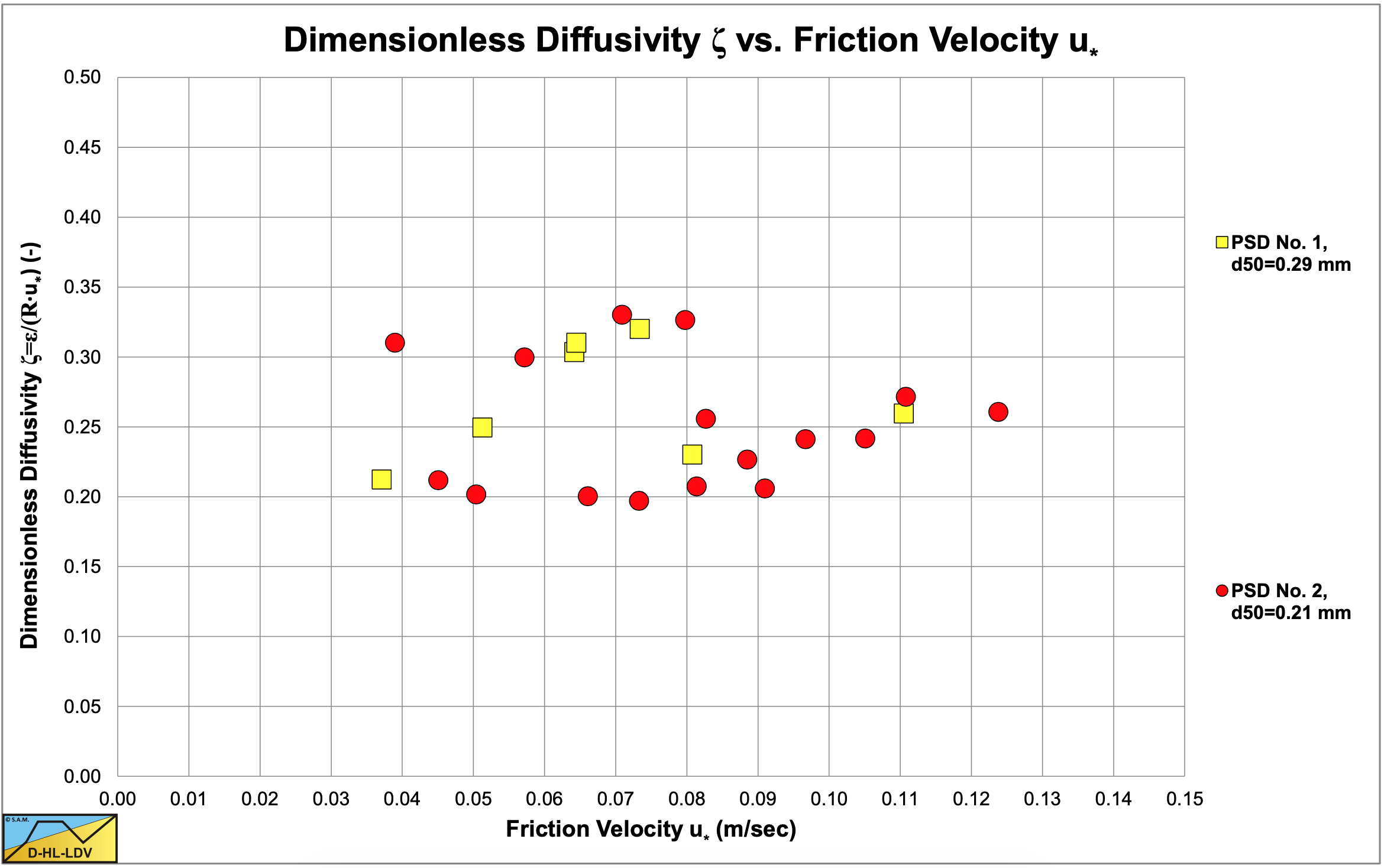
According to experiments of Matousek (2004) the mean diffusivity divided by the friction velocity and the pipe radius varies between 0.07 and 0.15, with no clear correlation with the mean delivered concentration (0.1-0.4) and the line speed (2-8 m/sec) in fine and medium sands.
\[\ \bar{\varepsilon}_{\mathrm{s}}=\frac{\beta_{\mathrm{sm}} \cdot \kappa \cdot \mathrm{u}_{*} \cdot \mathrm{D}_{\mathrm{p}}}{12}=\frac{\beta_{\mathrm{sm}} \cdot \kappa \cdot \mathrm{u}_{*} \cdot \mathrm{R}}{\mathrm{6}}
\Rightarrow \quad \frac{\bar{\varepsilon}_{\mathrm{s}}}{\mathrm{u}_{*} \cdot \mathrm{R}}=\frac{\beta_{\mathrm{sm}} \cdot \mathrm{\kappa}}{\mathrm{6}} \approx \mathrm{0 . 0 7} \quad\text{ for }\quad \beta_{\mathrm{sm}}=\mathrm{1} \quad\text{ and }\quad \mathrm{\kappa}=\mathrm{0 . 4}\]
Apparently the factor βsm linking sediment diffusivity to momentum diffusivity is larger than 1 for higher concentrations.
5.3.5.3 The Constant Diffusivity Approach for a Graded Sand
Karabelas (1977) applied the Hunt (1954) diffusion advection equation to pipe flow for a graded sand, but without hindered settling. Now suppose a graded sand can be divided into n fractions with z the vertical coordinate. The coordinate z is used, including the possibility of a bed. First equation (5.3-84) can be written as:
\[\ \mathrm{v}_{\mathrm{t}} \cdot \mathrm{C}_{\mathrm{v} \mathrm{s}}(\mathrm{z}) \cdot\left(1-\mathrm{C}_{\mathrm{v} \mathrm{s}}(\mathrm{z})\right)+\varepsilon_{\mathrm{s}} \cdot \frac{\partial \mathrm{C}_{\mathrm{v} \mathrm{s}}(\mathrm{z})}{\partial \mathrm{z}}=\mathrm{C}_{\mathrm{v} \mathrm{s}}(\mathrm{z}) \cdot\left(\mathrm{v}_{\mathrm{t}}-\mathrm{v}_{\mathrm{t}} \cdot \mathrm{C}_{\mathrm{v} \mathrm{s}}(\mathrm{z})\right)+\varepsilon_{\mathrm{s}} \cdot \frac{\partial \mathrm{C}_{\mathrm{v} \mathrm{s}}(\mathrm{z})}{\partial \mathrm{z}}
=\mathrm{C}_{\mathrm{v} \mathrm{s}}(\mathrm{z}) \cdot\left(\mathrm{v}_{\mathrm{t}}-\mathrm{v}_{\mathrm{l}}\right)+\varepsilon_{\mathrm{s}} \cdot \frac{\partial \mathrm{C}_{\mathrm{v} \mathrm{s}}(\mathrm{z})}{\partial \mathrm{z}}=\mathrm{0}\]
The advection diffusion equation for the jth fraction can now be written as:
\[\ \mathrm{C}_{\mathrm{v} \mathrm{s}, \mathrm{j}}(\mathrm{z}) \cdot\left(\mathrm{v}_{\mathrm{t}, \mathrm{j}}-\mathrm{v}_{\mathrm{l}}\right)+\varepsilon_{\mathrm{s}} \cdot \frac{\partial \mathrm{C}_{\mathrm{v} \mathrm{s}, \mathrm{j}}(\mathrm{z})}{\partial \mathrm{z}}=\mathrm{0}\]
The upwards liquid velocity vl is equal to the sum of the upwards velocities resulting from each fraction:
\[\ \mathrm{v}_{\mathrm{l}}=\sum_{\mathrm{i}=\mathrm{1}}^{\mathrm{n}} \mathrm{v}_{\mathrm{t}, \mathrm{i}} \cdot \mathrm{C}_{\mathrm{v} \mathrm{s}, \mathrm{i}}(\mathrm{z})\]
This gives for the advection diffusion equation of the jth fraction:
\[\ \mathrm{C}_{\mathrm{v s}, \mathrm{j}}(\mathrm{z}) \cdot\left(\mathrm{v}_{\mathrm{t}, \mathrm{j}}-\sum_{\mathrm{i}=\mathrm{1}}^{\mathrm{n}} \mathrm{v}_{\mathrm{t}, \mathrm{i}} \cdot \mathrm{C}_{\mathrm{v s}, \mathrm{i}}(\mathrm{z})\right)+\varepsilon_{\mathrm{s}} \cdot \frac{\partial \mathrm{C}_{\mathrm{v} \mathrm{s}, \mathrm{j}}(\mathrm{z})}{\partial \mathrm{z}}=\mathrm{0}\]
This results in a system of n coupled differential equations with the general mathematical solution:
\[\ \mathrm{C}_{\mathrm{v} \mathrm{s}, \mathrm{j}}(\mathrm{z})=\frac{\mathrm{G}_{\mathrm{j}} \cdot \mathrm{e}^{-\mathrm{v}_{\mathrm{t}, j} \cdot \mathrm{f}(\mathrm{z})}}{\mathrm{1}+\sum_{\mathrm{i}=1}^{\mathrm{n}} \mathrm{G}_{\mathrm{i}} \cdot \mathrm{e}^{-\mathrm{v}_{\mathrm{t}, \mathrm{i}} \cdot \mathrm{f}(\mathrm{z})}}
\quad \text {With : }\quad \mathrm{f}(\mathrm{z})=\int_{\mathrm{0}}^{\mathrm{z}} \frac{\mathrm{1}}{\varepsilon_{\mathrm{s}}(\mathrm{z})} \cdot \mathrm{d} \mathrm{z} \quad\text{ with: }\quad \varepsilon_{\mathrm{s}}(\mathrm{z})=\mathrm{c o n s t a n t} \quad \Rightarrow \quad \mathrm{f}(\mathrm{z})=\frac{\mathrm{z}}{\varepsilon_{\mathrm{s}}}\]
The variable Gj is a set of coefficients characteristic of each size fraction, but independent of the space coordinates. The assumption of a constant diffusivity is reasonable, except very close to the wall. For the diffusivity the following is chosen by Karabelas (1977):
\[\ \varepsilon_{\mathrm{s}}(\mathrm{z})=\zeta \cdot \mathrm{R} \cdot \mathrm{u}_{*}\]
Giving for the general solution:
\[\ \mathrm{C}_{\mathrm{v s}, \mathrm{j}}(\mathrm{z})=\frac{\mathrm{G}_{\mathrm{j}} \cdot \mathrm{e}^{-\frac{\mathrm{v}_{\mathrm{t}, \mathrm{j}}}{\zeta \cdot \mathrm{u}_{*}} \cdot \frac{\mathrm{z}}{\mathrm{R}}}}{1+\sum_{\mathrm{i}=1}^{\mathrm{n}} \mathrm{G}_{\mathrm{i}} \cdot \mathrm{e}^{-\frac{\mathrm{v}_{\mathrm{t}, \mathrm{i}}}{\zeta \cdot \mathrm{u}_{*}} \cdot \frac{\mathrm{z}}{\mathrm{R}}}}\]
For a uniform sand and no bed, using the Lane & Kalinske (1941) approach to determine the mean diffusivity, the solution, equation (5.3-85) is, with r starting at the bottom of the pipe:
\[\ \mathrm{C}_{\mathrm{v s}}(\mathrm{r})=\frac{\frac{\mathrm{C}_{\mathrm{v B}}}{\left(\mathrm{1 - C}_{\mathrm{v B}}\right)} \cdot \mathrm{e}^{-\frac{\mathrm{6 \cdot v _ { t }}}{\beta_{\mathrm{sm}} \cdot \mathrm{\kappa} \cdot \mathrm{u}_{*}} \cdot \frac{\mathrm{r}}{\mathrm{R}}}}{1+\frac{\mathrm{C}_{\mathrm{v B}}}{\left(\mathrm{1}-\mathrm{C}_{\mathrm{v B}}\right)} \cdot \mathrm{e}^{-\frac{\mathrm{6} \cdot \mathrm{v}_{\mathrm{t}}}{\beta_{\mathrm{sm}} \cdot \mathrm{\kappa} \cdot \mathrm{u}_{*}} \cdot \frac{r}{\mathrm{R}}}}\]
The equation for uniform sands has the same form as the equation for graded sands. The argument of the exponential power differs because a different diffusivity has been chosen using the Lane & Kalinske (1941) approach. Choosing the same mean diffusivity would give the same argument of the exponential power. Apparently one can write:
\[\ \mathrm{G}_{\mathrm{j}}=\frac{\mathrm{C}_{\mathrm{v} \mathrm{B}, \mathrm{j}}}{\left(1-\sum_{\mathrm{i}=1}^{\mathrm{n}} \mathrm{C}_{\mathrm{v} \mathrm{B}, \mathrm{j}}\right)}=\frac{\mathrm{C}_{\mathrm{v} \mathrm{B}, \mathrm{j}}}{\left(1-\mathrm{C}_{\mathrm{v} \mathrm{B}}\right)} \quad \text{ with: }\quad \sum_{\mathrm{i}=\mathrm{1}}^{\mathrm{n}} \mathrm{C}_{\mathrm{v} \mathrm{B}, \mathrm{j}}=\mathrm{C}_{\mathrm{v} \mathrm{B}}\]
So the variable Gj is related to the concentration CvB,j of the jth fraction at the bottom of the pipe. With:
\[\ \sum_{\mathrm{i}=1}^{\mathrm{n}} \mathrm{C}_{\mathrm{v} \mathrm{s}, \mathrm{i}}(\mathrm{z})=\sum_{\mathrm{i}=1}^{\mathrm{n}} \frac{\mathrm{G}_{\mathrm{i}} \cdot \mathrm{e}^{-\frac{\mathrm{v}_{\mathrm{t}, \mathrm{i}}}{\zeta \cdot \mathrm{u}_{*}} \cdot \frac{\mathrm{z}}{\mathrm{R}}}}{\mathrm{1}+\sum_{\mathrm{i}=\mathrm{1}}^{\mathrm{n}} \mathrm{G}_{\mathrm{i}} \cdot \mathrm{e}^{-\frac{\mathrm{v}_{\mathrm{t}, \mathrm{i}}}{\zeta \cdot \mathrm{u}_{*}} \cdot \frac{\mathrm{z}}{\mathrm{R}}}}=\frac{\sum_{\mathrm{i}=\mathrm{1}}^{\mathrm{n}} \mathrm{G}_{\mathrm{i}} \cdot \mathrm{e}^{-\frac{\mathrm{v}_{\mathrm{t}}, \mathrm{i}}{\zeta \cdot \mathrm{u}_{*}} \cdot \frac{\mathrm{z}}{\mathrm{R}}}}{\mathrm{1}+\sum_{\mathrm{i}=\mathrm{1}}^{\mathrm{n}} \mathrm{G}_{\mathrm{i}} \cdot \mathrm{e}^{-\frac{\mathrm{v}_{\mathrm{t}, \mathrm{i}}}{\zeta \cdot \mathrm{u}_{*}} \cdot \frac{\mathrm{z}}{\mathrm{R}}}}\]
One can write:
\[\ \begin{array} \sum_{\mathrm{i}=1}^{\mathrm{n}} \mathrm{C}_{\mathrm{v} \mathrm{s}, \mathrm{i}}(\mathrm{z}) \cdot\left(\mathrm{1}+\sum_{\mathrm{i}=\mathrm{1}}^{\mathrm{n}} \mathrm{G}_{\mathrm{i}} \cdot \mathrm{e}^{-\frac{\mathrm{v}_{\mathrm{t}, \mathrm{i}}}{\zeta \cdot \mathrm{u}_{*}} \cdot \frac{\mathrm{z}}{\mathrm{R}}}\right)=\sum_{\mathrm{i}=\mathrm{1}}^{\mathrm{n}} \mathrm{G}_{\mathrm{i}} \cdot \mathrm{e}^{-\frac{\mathrm{v}_{\mathrm{t}, \mathrm{i}}}{\zeta \cdot \mathrm{u}_{*}} \cdot \frac{\mathrm{z}}{\mathrm{R}}}\\
\sum_{\mathrm{i}=\mathrm{1}}^{\mathrm{n}} \mathrm{C}_{\mathrm{v} \mathrm{s}, \mathrm{i}}(\mathrm{z})=\sum_{\mathrm{i}=1}^{\mathrm{n}} \mathrm{G}_{\mathrm{i}} \cdot \mathrm{e}^{-\frac{\mathrm{v}_{\mathrm{t}, \mathrm{i}}}{\zeta \cdot \mathrm{u}_{*}} \cdot \frac{\mathrm{z}}{\mathrm{R}}} \cdot\left(1-\sum_{\mathrm{i}=1}^{\mathrm{n}} \mathrm{C}_{\mathrm{v} \mathrm{s}, \mathrm{i}}(\mathrm{z})\right)\\
\left.\frac{\sum_{\mathrm{i}=\mathrm{1}}^{\mathrm{n}} \mathrm{C}_{\mathrm{v} \mathrm{s}, \mathrm{i}}(\mathrm{z})}{\left(\mathrm{1}-\sum_{\mathrm{i}=\mathrm{1}}^{\mathrm{n}} \mathrm{C}_{\mathrm{v} \mathrm{s}, \mathrm{i}} \mathrm{( z}\right)}\right)=\sum_{\mathrm{i}=1}^{\mathrm{n}} \mathrm{G}_{\mathrm{i}} \cdot \mathrm{e}^{-\frac{\mathrm{v}_{\mathrm{t}, \mathrm{i}}}{\zeta \cdot \mathrm{u}_{*}} \cdot \frac{\mathrm{z}}{\mathrm{R}}}\end{array}\]
Or:
\[\ \frac{\mathrm{C}_{\mathrm{v} \mathrm{s}, \mathrm{j}}(\mathrm{z})}{\left(1-\sum_{\mathrm{i}=\mathrm{1}}^{\mathrm{n}} \mathrm{C}_{\mathrm{v} \mathrm{s}, \mathrm{i}} \mathrm{( z )}\right)}=\mathrm{G}_{\mathrm{j}} \cdot \mathrm{e}^{-\frac{\mathrm{v}_{\mathrm{t}, \mathrm{j}}}{\zeta \cdot \mathrm{u}_{*}} \frac{\mathrm{z}}{\mathrm{R}}}\]
For the bottom of the pipe where z=0 this gives:
\[\ \mathrm{G}_{\mathrm{j}}=\frac{\mathrm{C}_{\mathrm{v s}, \mathrm{j}}(\mathrm{0})}{\left(1-\sum_{\mathrm{i}=\mathrm{1}}^{\mathrm{n}} \mathrm{C}_{\mathrm{v s}, \mathrm{i}} \mathrm{( 0 )}\right)}=\frac{\mathrm{C}_{\mathrm{v B}, \mathrm{j}}}{\left(1-\sum_{\mathrm{i}=\mathrm{1}}^{\mathrm{n}} \mathrm{C}_{\mathrm{v} \mathrm{B}, \mathrm{i}}\right)}=\frac{\mathrm{C}_{\mathrm{v} \mathrm{B}, \mathrm{j}}}{\left(\mathrm{1}-\mathrm{C}_{\mathrm{v} \mathrm{B}}\right)}\]
Proving that equation (5.3-93) can also be written as:
\[\ \mathrm{C}_{\mathrm{v s}, \mathrm{j}}(\mathrm{z})=\frac{\frac{\mathrm{C}_{\mathrm{v} \mathrm{B}, \mathrm{j}}}{\left(\mathrm{1}-\mathrm{C}_{\mathrm{v} \mathrm{B}}\right)} \cdot \mathrm{e}^{-\frac{\mathrm{v}_{\mathrm{t}, \mathrm{j}}}{\zeta \cdot \mathrm{u}_{*}} \cdot \frac{\mathrm{z}}{\mathrm{R}}}}{1+\sum_{\mathrm{i}=1}^{\mathrm{n}} \frac{\mathrm{C}_{\mathrm{v} \mathrm{B}, \mathrm{i}}}{\left(\mathrm{1}-\mathrm{C}_{\mathrm{v} \mathrm{B}}\right)} \cdot \mathrm{e}^{-\frac{\mathrm{v}_{\mathrm{t}, \mathrm{i}}}{\zeta \cdot \mathrm{u}_{*}} \cdot \frac{\mathrm{z}}{\mathrm{R}}}}\]
With CvB,j the concentration of the jth fraction at the bottom of the pipe and CvB the total bottom concentration. Assuming that the mean concentration of each fraction is known a priori and the total mean concentration is known a priori, equation (5.3-98) can be written as:
\[\ \frac{\mathrm{C}_{\mathrm{v s}, \mathrm{j}}}{\left(\mathrm{1 - C}_{\mathrm{v s}}\right)}=\mathrm{G}_{\mathrm{j}} \cdot \frac{\mathrm{1}}{\mathrm{A}} \cdot \int_{\mathrm{A}} \mathrm{e}^{-\frac{\mathrm{v}_{\mathrm{t}, \mathrm{j}}}{\zeta \cdot \mathrm{u}_{*}}\cdot \frac{\mathrm{z}}{\mathrm{R}}} \cdot \mathrm{d} \mathrm{A}\]
Giving for Gj according to Karabelas (1977):
\[\ \mathrm{G}_{\mathrm{j}}=\frac{\mathrm{C}_{\mathrm{v} s, \mathrm{j}}}{\left(1-\mathrm{C}_{\mathrm{v} \mathrm{s}}\right)} \cdot \frac{\mathrm{1}}{\frac{1}{\mathrm{A}} \cdot \int_{\mathrm{A}} \mathrm{e}^{-\frac{\mathrm{v}_{\mathrm{t}, \mathrm{j}}}{\zeta \cdot \mathrm{u}_{*}}\cdot{\frac{\mathrm{z}}{ \mathrm{R}}}}{ \cdot \mathrm{d} \mathrm{A}}}=\frac{\mathrm{C}_{\mathrm{v} \mathrm{s}, \mathrm{j}}}{\left(1-\mathrm{C}_{\mathrm{v} \mathrm{s}}\right)} \cdot \frac{\mathrm{1}}{\mathrm{E}_{\mathrm{j}}} \quad
\text{With : }\quad \mathrm{E}_{\mathrm{j}} \approx \mathrm{1}+\frac{\left(\frac{\mathrm{v}_{\mathrm{t}, \mathrm{j}}}{\zeta \cdot \mathrm{u}_{*}}\right)^{2}}{\mathrm{8}} \cdot\left(1+\frac{\left(\frac{\mathrm{v}_{\mathrm{t}, \mathrm{j}}}{\zeta \cdot \mathrm{u}_{*}}\right)^{2}}{\mathrm{2 4}}\right)\]
This solution is valid for a constant diffusivity over the pipe cross section and no hindered settling.
For the case of one dimensional open channel flow with height H, Karabelas (1977) gives:
\[\ \mathrm{G}_{\mathrm{j}}=\frac{\mathrm{C}_{\mathrm{v} s, \mathrm{j}}}{\left(1-\mathrm{C}_{\mathrm{v} \mathrm{s}}\right)} \cdot \frac{\mathrm{1}}{\frac{\mathrm{1}}{\mathrm{H}} \cdot \int_{\mathrm{0}}^{\mathrm{H}} \mathrm{e}^{-\frac{\mathrm{v}_{\mathrm{t}, \mathrm{j}}}{\zeta \cdot \mathrm{u}_{*}} \cdot \frac{\mathrm{z}}{\mathrm{H}}} \cdot \mathrm{d} \mathrm{z}}\]
Giving for the general solution:
\[\ \mathrm{C}_{\mathrm{v s}, \mathrm{j}}(\mathrm{z})=\frac{\mathrm{G}_{\mathrm{j}} \cdot \mathrm{e}^{-\frac{\mathrm{v}_{\mathrm{t}, \mathrm{j}}}{\zeta \cdot \mathrm{u}_{*}} \cdot \frac{\mathrm{z}}{\mathrm{H}}}}{\mathrm{1}+\sum_{\mathrm{i}=1}^{\mathrm{n}} \mathrm{G}_{\mathrm{i}} \cdot \mathrm{e}^{-\frac{\mathrm{v}_{\mathrm{t}, \mathrm{i}}}{\zeta \cdot \mathrm{u}_{*}} \cdot \frac{\mathrm{z}}{\mathrm{H}}}}\]
5.3.6 Conclusions & Discussion Pipe Flow
For pipe flow the constant lateral diffusivity approach for uniform sands is a good first approximation using the mean diffusivity divided by the friction velocity and the pipe radius ζ with values larger than the theoretical expected values. Karabelas (1977) found an average value of 0.255, which is 3 to 4 times larger than the diffusivity of liquid in the absence of particles. The median particle diameter was nearly equal to the Kolmogorov micro scale of turbulence. Other researchers have used spherical particles with diameters one to two magnitudes larger than the Kolmogorov micro scale of turbulence and found slightly higher diffusivities between 0.3 and 0.4.
The Karabelas (1977) method for graded sands is a good starting point and has been used by several researchers to develop more sophisticated methods, which will be described in chapter 6. The open channel approach of Karabelas (1977) is a good first guess of the parameter Gj. For very small particles this results in an average concentration equal to the concentration at the bottom, meaning homogeneous flow.
\[\ \mathrm{G}_{\mathrm{j}}=\frac{\mathrm{C}_{\mathrm{v B}, \mathrm{j}}}{\left(1-\mathrm{C}_{\mathrm{v B}}\right)}\]
For a uniform sand this gives:
\[\ \mathrm{C}_{\mathrm{v} \mathrm{B}, \mathrm{j}}=\frac{\mathrm{1}-\mathrm{e}^{-\overline{\mathrm{C}}_{\mathrm{v}_{s}, \mathrm{j}} \cdot \frac{\mathrm{v}_{\mathrm{t}, \mathrm{j}} \cdot \mathrm{H}}{\varepsilon_{\mathrm{s}}}}}{\mathrm{1 - e}^{-\frac{\mathrm{v}_{\mathrm{t}} \cdot \mathrm{H}}{\varepsilon_{\mathrm{s}}}}}\]
Figure 5.3-3 and Figure 5.3-4 show concentration profiles from Karabelas (1977), compared with profiles determined with equation (5.3-70) for open channel flow and uniform sand with H=Dp. It should be mentioned that the concentration were very low, 0.3%, so there was no hindered settling. The reason for comparing a graded sand in pipe flow with a uniform sand in open channel flow is, to see if the relatively simple analytical solution gives a good approximation, which it does. The higher the line speed, the better the approximation.
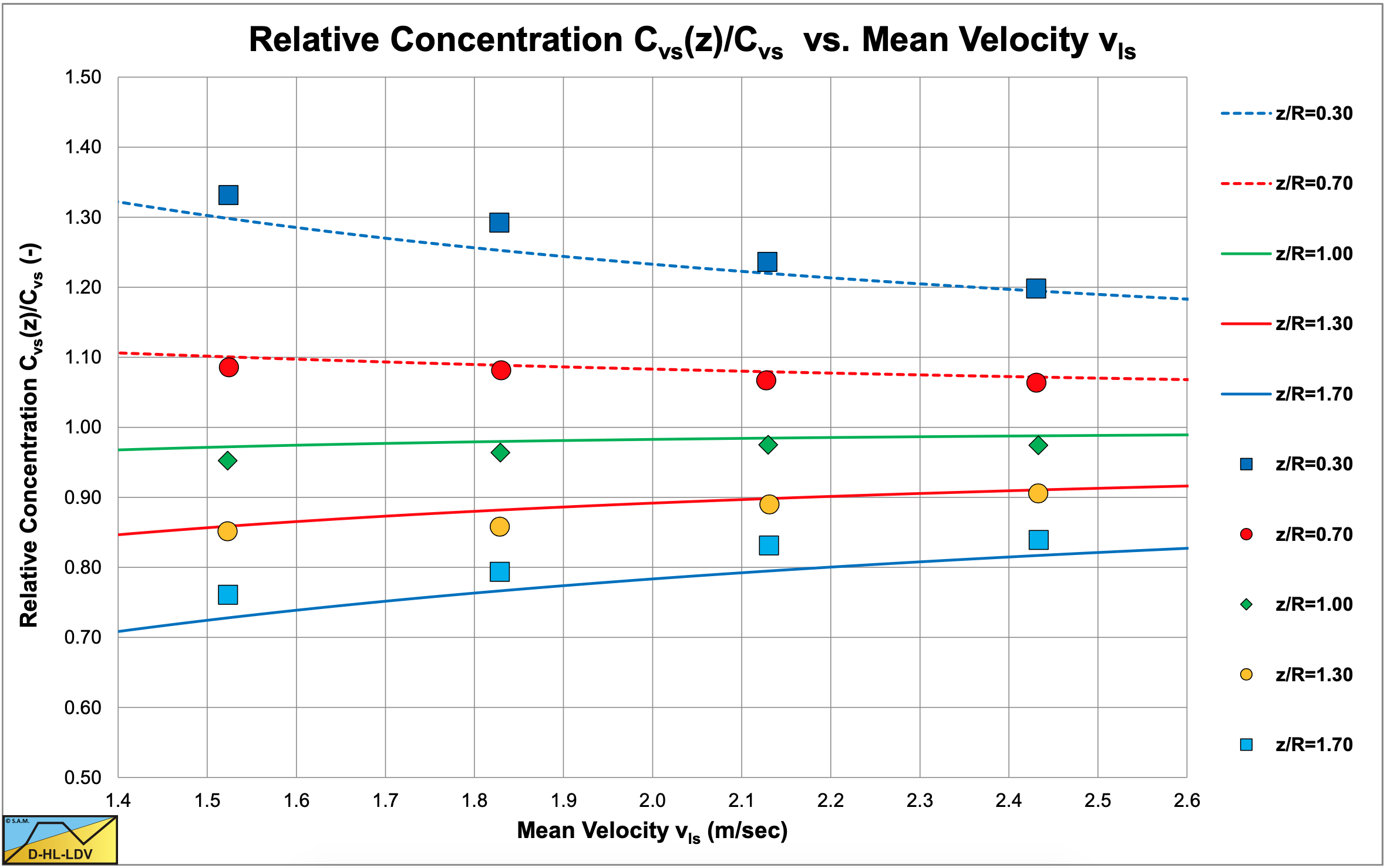
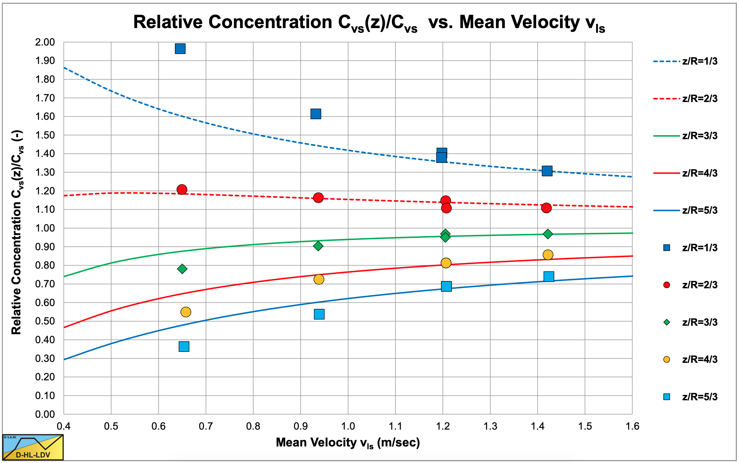
5.3.7 Nomenclature Erosion, Bed Load and Suspended Load
|
a |
Elevation above the bed |
m |
|
Bs |
Factor in Hunt equation | - |
| C | Volumetric concentration | - |
|
Cvs(z) |
Volumetric concentration | - |
|
Cvs,sf |
Volumetric concentration in sheet flow layer | - |
|
Cvb |
Volumetric concentration bed | - |
|
CvB |
Volumetric concentration bottom of channel or pipe | - |
|
Cvl |
Volumetric concentration liquid | - |
|
d |
Particle diameter |
m |
|
Dp |
Pipe diameter | m |
|
E |
Coefficient in Karabelas approach |
- |
|
f(z) |
Function related to diffusivity integration |
s/m |
|
g |
Gravitational constant (9.81 m/s2) |
m/s2 |
|
G |
Coefficient in Karabelas approach |
- |
|
H |
Height of the flow layer |
m |
|
H |
Thickness sheet flow layer |
m |
|
i, j |
Fraction number |
- |
|
n |
Number of fractions |
- |
|
n |
Power used for velocity profile in sheet flow layer |
- |
|
P |
Rouse number |
- |
|
qb |
Bed load transport |
m2/s |
|
qs,down |
Downwards flow of particles |
1/s |
|
qs,up |
Upwards flow of particles |
1/s |
|
Qs |
Total sediment transport or bed load |
m3/s |
|
r |
Vertical coordinate in pipe |
m |
|
R |
Radius of pipe |
m |
|
Rsd |
Relative submerged density (about 1.65 for sand) |
- |
|
t |
Time |
s |
|
u* |
Friction velocity |
m/s |
|
U(z) |
Velocity in the flow layer or in sheet flow layer |
m/s |
|
UH |
Velocity at top sheet flow layer |
m/s |
|
Umean |
Mean velocity in sheet flow layer |
m/s |
|
u |
Velocity in x direction |
m/s |
|
v |
Velocity in y direction |
m/s |
|
vl |
Vertical velocity liquid upwards |
m/s |
|
vs |
Vertical velocity solids or sediment downwards |
m/s |
|
vt |
Terminal settling velocity |
m/s |
|
w |
Velocity in z direction |
m/s |
|
w |
Bed width |
m |
|
x |
Coordinate |
m |
|
y |
Coordinate |
m |
|
z |
Coordinate |
m |
|
z |
Vertical position in the flow layer |
m |
|
z0 |
Starting point logarithmic velocity profile |
m |
|
z1 |
Ordinate Rouse profile |
m |
|
α |
Coefficient MPM equation (usually 8) |
- |
|
β |
Power MPM equation (usually 1.5) |
- |
|
β |
Richardson & Zaki power hindered settling |
- |
|
βsm |
Relation sediment mass diffusivity to eddy momentum diffusivity |
- |
|
εm |
Diffusivity molecular |
m/s |
|
εm |
Eddy momentum diffusivity |
m/s |
|
εs |
Sediment diffusivity |
m/s |
|
εsx |
Diffusivity turbulent x direction sediment |
m/s |
|
εsy |
Diffusivity turbulent y direction sediment |
m/s |
|
εsz |
Diffusivity turbulent z direction sediment |
m/s |
|
εlz |
Diffusivity turbulent z direction liquid |
m/s |
| \(\ \boldsymbol{\gamma}\) |
Coefficient velocity top sheet flow layer |
- |
|
λb |
Bed Darcy Weisbach friction factor |
- |
|
κ, κs |
von Karman constant |
- |
|
φ |
Internal friction angle bed |
rad |
|
ρl |
Liquid density |
ton/m3 |
|
θ |
Shields parameter or dimensionless shear stress | - |
| θcr | Critical Shields parameter | - |
|
\(\ \mathrm{\boldsymbol{\tau}(z)}\) |
Shear stress as function of vertical coordinate |
Pa |
| \(\ \mathrm{\boldsymbol{\tau}_b}\) |
Bed shear stress |
Pa |
|
Φb |
Dimensionless bed load transport |
- |
|
ζ |
Rouse number |
- |
|
ζ |
Relation sediment mass diffusivity to eddy momentum diffusivity in Karabelas - approach |
- |