
6.25: Talmon (2011) and (2013) Homogeneous Regime
- Page ID
- 31499

6.25.1 Theory
Talmon (2013) derived an equation to correct the homogeneous equation (the ELM model) for the slurry density, based on the hypothesis that the viscous sub-layer hardly contains solids at very high line speeds in the homogeneous regime. This theory results in a reduction of the resistance compared with the ELM, but the resistance is still higher than the resistance of clear water. Talmon (2013) used the Prandl approach for the mixing length, which is a 2D approach for open channel flow with a free surface. The Prandl approach was extended with damping near the wall to take into account the viscous effects near the wall, according to von Driest (Schlichting, 1968):
\[\ \begin{array}{left} \text{Prandl: }\quad \ell=\kappa \cdot \mathrm{z}\\
\text{von Driest : }\ell=\kappa \cdot \mathrm{z} \cdot\left(1-\mathrm{e}^{-\mathrm{z}^{+} / \mathrm{A}}\right) \quad\text{ with: }\quad \mathrm{z}^{+}=\frac{\mathrm{z} \cdot \mathrm{u}_{*}}{v_{\mathrm{l}}} \quad \mathrm{A}=\mathrm{2} \mathrm{6}\end{array}\]
The shear stress between the mixture, the slurry, and the pipe wall is the sum of the viscous shear stress and the turbulent shear stress:
\[\ \begin{array}{left}\tau=\tau_{v}+\tau_{\mathrm{t}}=\mu_{v} \cdot \frac{\partial \mathrm{u}}{\partial \mathrm{z}}+\mu_{\mathrm{t}} \cdot \frac{\partial \mathrm{u}}{\partial \mathrm{z}}=\rho_{\mathrm{m}} \cdot v_{\mathrm{m}} \cdot \frac{\partial \mathrm{u}}{\partial \mathrm{z}}+\rho_{\mathrm{m}} \cdot v_{\mathrm{t}} \cdot \frac{\partial \mathrm{u}}{\partial \mathrm{z}}\\
\text{With for the eddy viscosity : }\\
v_{\mathrm{t}}=\ell^{2} \cdot\left|\frac{\partial \mathrm{u}}{\partial \mathrm{z}}\right|\end{array}\]
So the shear stress can be expressed as:
\[\ \tau=\rho_{\mathrm{m}} \cdot\left(\mathrm{u}_{*}\right)^{2}=\rho_{\mathrm{m}} \cdot\left(v_{\mathrm{m}}+\ell^{2} \cdot\left|\frac{\partial \mathrm{u}}{\partial \mathrm{z}}\right|\right) \cdot \frac{\partial \mathrm{u}}{\partial \mathrm{z}}\]
Solving this with respect to the velocity gradient gives:
\[\ \frac{\partial \mathrm{u}}{\partial \mathrm{z}}=\frac{-\frac{\mu_{\mathrm{m}}}{\rho_{\mathrm{m}}}+\sqrt{\left(\frac{\mu_{\mathrm{m}}}{\rho_{\mathrm{m}}}\right)^{2}+4 \cdot \ell^{2} \cdot\left(\mathrm{u}_{*}\right)^{2}}}{2 \cdot \ell^{2}}=\frac{2 \cdot\left(\mathrm{u}^{*}\right)^{2}}{\frac{\mu_{\mathrm{m}}}{\rho_{\mathrm{m}}}+\sqrt{\left(\frac{\mu_{\mathrm{m}}}{\rho_{\mathrm{m}}}\right)^{2}+4 \cdot \ell^{2} \cdot\left(\mathrm{u}_{*}\right)^{2}}}\]
Assuming that the term with the density ratio is relevant only near the pipe wall and not in the center of the pipe, this equation will simulate a mixture with liquid in the viscous sub-layer. In fact, the density ratio reduces the effect of the kinematic viscosity, which mainly affects the viscous sub-layer. The velocity difference um-ufl can now be determined with:
\[\ \mathrm{u}_{\mathrm{m}}-\mathrm{u}_{\mathrm{l}}=\int_{\mathrm{0}}^{\mathrm{z}_{\max }} \frac{-\frac{\rho_{\mathrm{l}}}{\rho_{\mathrm{m}}} \cdot v_{\mathrm{l}}+\sqrt{\left(\frac{\rho_{\mathrm{l}}}{\rho_{\mathrm{m}}} \cdot v_{\mathrm{l}}\right)^{2}+4 \cdot \ell^{2} \cdot\left(\mathrm{u}_{*}\right)^{2}}}{2 \cdot \ell^{2}} \cdot \mathrm{d} \mathrm{z}-\int_{\mathrm{0}}^{\mathrm{z}_{\max }} \frac{-v_{\mathrm{l}}+\sqrt{\left(v_{\mathrm{l}}\right)^{2}+4 \cdot \ell^{2} \cdot\left(\mathrm{u}_{*}\right)^{2}}}{2 \cdot \ell^{2}} \cdot \mathrm{d} \mathrm{z}\]
This velocity difference, in the center of the pipe is about equal to the difference of the average line speeds. Further it appears that dividing the velocity difference by the friction velocity results in a factor F, which only depends on the volumetric concentration Cvs, the relative submerged density Rsd, slightly on the line speed vls in the range 3- 10 m/sec and on the pipe diameter Dp, according to:
\[\ \mathrm{F}=\frac{\mathrm{u}_{\mathrm{m}}-\mathrm{u}_{\mathrm{l}}}{\mathrm{u}_{*}}=\frac{\mathrm{v}_{\mathrm{l} \mathrm{s}, \mathrm{m}}-\mathrm{v}_{\mathrm{l} \mathrm{s}, \mathrm{l}}}{\mathrm{u}_{*}}=\alpha_{\mathrm{h}} \cdot \mathrm{R}_{\mathrm{s} \mathrm{d}} \cdot \mathrm{C}_{\mathrm{v} \mathrm{s}}=\alpha_{\mathrm{h}} \cdot\left(\frac{\rho_{\mathrm{m}}}{\rho_{\mathrm{l}}}-\mathrm{1}\right)\]
The shear stress at the pipe wall of a Newtonian liquid is by definition:
\[\ \rho_{\mathrm{l}} \cdot\left(\mathrm{u}_{*}\right)^{2}=\frac{\lambda_{\mathrm{l}}}{\mathrm{8}} \cdot \rho_{\mathrm{l}} \cdot \mathrm{v}_{\mathrm{l} \mathrm{s}, \mathrm{l}}^{2} \quad\text{ and }\quad \rho_{\mathrm{m}} \cdot\left(\mathrm{u}_{*}\right)^{2}=\frac{\lambda_{\mathrm{m}}}{\mathrm{8}} \cdot \rho_{\mathrm{m}} \cdot \mathrm{v}_{\mathrm{ls}, \mathrm{m}}^{2}\]
From this a relation for the ratio of the Moody friction coefficients of a flow with mixture in the center and carrier liquid in the viscous sub-layer to a flow with 100% liquid can be derived.
\[\ \frac{\lambda_{\mathrm{l}}}{8} \cdot \mathrm{v}_{\mathrm{ls, l}}^{2}=\frac{\lambda_{\mathrm{m}}}{8} \cdot \mathrm{v}_{\mathrm{ls}, \mathrm{m}}^{2} \Rightarrow \frac{\lambda_{\mathrm{m}}}{\lambda_{\mathrm{l}}}=\frac{\mathrm{v}_{\mathrm{ls}, \mathrm{l}}^{2}}{\mathrm{v}_{\mathrm{ls}, \mathrm{m}}^{2}} \Rightarrow \frac{\lambda_{\mathrm{m}}}{\lambda_{\mathrm{l}}}=\frac{\mathrm{v}_{\mathrm{ls, l}}^{2}}{\left(\mathrm{F} \cdot \mathrm{u}_{*}+\mathrm{v}_{\mathrm{ls, l}}\right)^{2}}=\frac{1}{\left(\mathrm{F} \cdot \mathrm{u}_{*}+1\right)^{2}}\]
The Talmon (2013) approach resulted in the following equation:
\[\ \frac{\lambda_{\mathrm{m}}}{\lambda_{\mathrm{l}}}=\frac{\mathrm{1}}{\left(\mathrm{F} \cdot \frac{\mathrm{u}_{*}}{\mathrm{v}_{\mathrm{l} \mathrm{s}, \mathrm{l}}}+\mathrm{1}\right)^{2}}=\frac{\mathrm{1}}{\left(\alpha_{\mathrm{h}} \cdot \sqrt{\frac{\lambda_{\mathrm{l}}}{\mathrm{8}}}{ \cdot \mathrm{R}_{\mathrm{s d}} \cdot \mathrm{C}_{\mathrm{v s}}+\mathrm{1}}\right)^{\mathrm{2}}}\]
The resulting equation is:
\[\ \frac{\mathrm{i}_{\mathrm{m}}}{\mathrm{i}_{\mathrm{l}}}=\frac{\mathrm{1}+\mathrm{R}_{\mathrm{s d}} \cdot \mathrm{C}_{\mathrm{v s}}}{(\alpha_{\mathrm{h}} \cdot \sqrt{\frac{\lambda_{\mathrm{l}}}{\mathrm{8}}}{ \cdot \mathrm{R}_{\mathrm{s d}} \cdot \mathrm{C}_{\mathrm{v s}}+\mathrm{1})^{2}}} \Rightarrow \mathrm{i}_{\mathrm{m}}=\mathrm{i}_{\mathrm{l}} \cdot \frac{\mathrm{1}+\mathrm{R}_{\mathrm{s d}} \cdot \mathrm{C}_{\mathrm{v s}}}{\left(\alpha_{\mathrm{h}} \cdot \sqrt{\frac{\lambda_{\mathrm{l}}}{\mathrm{8}}}{ \cdot \mathrm{R}_{\mathrm{s d}} \cdot \mathrm{C}_{\mathrm{v s}}+\mathrm{1}}\right)^{2}}\]
In order to find the relative excess hydraulic gradient Erhg, this can be written as:
\[\ \begin{array}{left} \mathrm{i}_{\mathrm{m}}-\mathrm{i}_{\mathrm{l}}&=\mathrm{i}_{\mathrm{l}} \cdot \frac{\mathrm{1}+\mathrm{R}_{\mathrm{s} \mathrm{d}} \cdot \mathrm{C}_{\mathrm{v} \mathrm{s}}}{\left(\alpha_{\mathrm{h}} \cdot \sqrt{\frac{\lambda_{\mathrm{l}}}{\mathrm{8}}}{ \cdot \mathrm{R}_{\mathrm{s d}} \cdot \mathrm{C}_{\mathrm{v s}}+\mathrm{1}}\right)^{2}}{-\mathrm{i}_{\mathrm{l}} \cdot \frac{\left(\alpha_{\mathrm{h}} \cdot \sqrt{\frac{\lambda_{\mathrm{l}}}{\mathrm{8}}}{ \cdot \mathrm{R}_{\mathrm{s d}} \cdot \mathrm{C}_{\mathrm{v s}}+1}\right)^{2}}{\left(\alpha_{\mathrm{h}} \cdot \sqrt{\frac{\lambda_{\mathrm{l}}}{\mathrm{8}}}{ \cdot \mathrm{R}_{\mathrm{s d}} \cdot \mathrm{C}_{\mathrm{v s}}+1}\right)^{2}}}\\
&=\mathrm{i}_{\mathrm{l}} \cdot \frac{\mathrm{R}_{\mathrm{sd}} \cdot \mathrm{C}_{\mathrm{vs}}+1-\left(\alpha_{\mathrm{h}} \cdot \sqrt{\frac{\lambda_{\mathrm{l}}}{8}} \cdot \mathrm{R}_{\mathrm{sd}} \cdot \mathrm{C}_{\mathrm{vs}}+1\right)^{2}}{\left(\alpha_{\mathrm{h}} \cdot \sqrt{\frac{\lambda_{\mathrm{l}}}{8}}{ \cdot \mathrm{R}_{\mathrm{sd}} \cdot \mathrm{C}_{\mathrm{vs}}+1}\right)^{2}}\end{array}
\]
The relative excess hydraulic gradient Erhg is now:
\[\ \mathrm{E}_{\mathrm{r h g}}=\frac{\mathrm{i}_{\mathrm{m}}-\mathrm{i}_{\mathrm{l}}}{\mathrm{R}_{\mathrm{s d}} \cdot \mathrm{C}_{\mathrm{v s}}}=\mathrm{i}_{\mathrm{l}} \cdot \frac{\mathrm{R}_{\mathrm{s d}} \cdot \mathrm{C}_{\mathrm{v s}}+\mathrm{1}-\left(\alpha_{\mathrm{h}} \cdot \sqrt{\frac{\lambda_{\mathrm{l}}}{\mathrm{8}}}{ \cdot \mathrm{R}_{\mathrm{s d}} \cdot \mathrm{C}_{\mathrm{v s}}+\mathrm{1}}\right)^{2}}{\mathrm{R}_{\mathrm{s d}} \cdot \mathrm{C}_{\mathrm{v s}} \cdot\left(\alpha_{\mathrm{h}} \cdot \sqrt{\frac{\lambda_{\mathrm{l}}}{\mathrm{8}}}{ \cdot \mathrm{R}_{\mathrm{s d}} \cdot \mathrm{C}_{\mathrm{v s}}+\mathrm{1}}\right)^{2}}\]
The limiting value for the excess hydraulic gradient Erhg for a volumetric spatial concentration Cvs approaching zero, becomes irrespective of the relative submerged density Rsd:
\[\ \mathrm{E}_{\mathrm{rhg}}=\frac{\mathrm{i}_{\mathrm{m}}-\mathrm{i}_{\mathrm{l}}}{\mathrm{R}_{\mathrm{sd}} \cdot \mathrm{C}_{\mathrm{vs}}}=\mathrm{i}_{\mathrm{l}} \cdot\left(1-2 \cdot \alpha_{\mathrm{h}} \cdot \sqrt{\frac{\lambda_{\mathrm{l}}}{8}}\right)\]
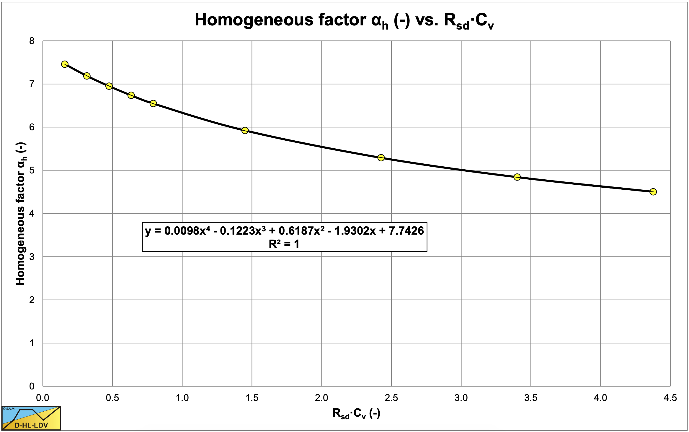
Figure 6.25-1 shows the factor αh as a function of the term Rsd·Cvs. The value of this coefficient decreases with increasing density according to:
\[\ \alpha_{\mathrm{h}}=7.7426-1.9302 \cdot\left(\mathrm{R}_{\mathrm{sd}} \cdot \mathrm{C}_{\mathrm{vs}}\right)+0.6187 \cdot\left(\mathrm{R}_{\mathrm{sd}} \cdot \mathrm{C}_{\mathrm{vs}}\right)^{2}
-\mathrm{0.1223} \cdot\left(\mathrm{R}_{\mathrm{sd}} \cdot \mathrm{C}_{\mathrm{vs}}\right)^{3}+0.0098 \cdot\left(\mathrm{R}_{\mathrm{sd}} \cdot \mathrm{C}_{\mathrm{vs}}\right)^{4}\]
Talmon (2013) used αh=6.7 as a fixed value. The model underestimates the hydraulic gradient in a number of cases (small and large particles) as Talmon (2013) proves with the examples shown in his paper. Only for d50=0.37 mm and Dp=0.15 m (medium particles) there is a good match. The philosophy behind this theory, combining a viscous sub-layer with water with a kernel with mixture, is however very interesting, because it explains fundamentally why the pressure can be lower than the pressure according to the ELM, as has been shown by many researchers. The model has been derived using the standard mixing length equation for 2D flow. Applying the Nikuradse (1933) equation for the mixing length in pipe flow may give different quantitative results.
6.25.2 Nomenclature Talmon Model
|
A |
Von Driest damping factor (26) |
- |
|
Dp |
Pipe diameter |
m |
|
Erhg |
Relative excess hydraulic gradient |
- |
|
F |
Homogeneous reduction factor |
- |
|
g |
Gravitational constant (9.81) |
m/s2 |
|
ΔL |
Length of pipe segment considered |
m |
|
im |
Mixture hydraulic gradient |
m/m |
|
il |
Liquid hydraulic gradient |
m/m |
|
Rsd |
Relative submerged density (sand 1.65) |
- |
|
u |
Velocity |
m/s |
|
ul |
Velocity liquid |
m/s |
|
um |
Velocity mixture |
m/s |
|
u* |
Friction velocity |
m/s |
|
vls |
Line speed |
m/s |
|
vls,l |
Line speed liquid |
m/s |
|
vls,m |
Line speed mixture |
m/s |
|
z |
Distance to the wall |
m |
|
αh |
Homogeneous factor |
- |
|
λl |
Darcy-Weisbach friction factor liquid |
- |
|
λm |
Darcy-Weisbach friction factor mixture |
- |
|
ρl |
Density liquid |
ton/m3 |
|
ρm |
Density mixture |
ton/m3 |
|
κ |
Von Karman constant (0.4) |
- |
| \(\ \mathrm{\tau}\) |
Shear stress |
kPa |
| \(\ \tau_\mathrm{v}\) |
Viscous shear stress |
kPa |
| \(\ \tau_{\mathrm{t}}\) |
Turbulent shear stress |
kPa |
|
μν |
Viscous dynamic viscosity |
Pa·s |
|
μt |
Turbulent dynamic viscosity |
Pa·s |
|
μl |
Dynamic viscosity liquid |
Pa·s |
|
μm |
Dynamic viscosity mixture |
Pa·s |
|
νl |
Kinematic viscosity liquid |
m2/s |
|
νm |
Kinematic viscosity mixture |
m2/s |
|
νt |
Turbulence viscosity |
m2/s |
| \(\ \boldsymbol{\ell}\) |
Mixing length |
m |