
6.27: The Limit Deposit Velocity (LDV)
- Page ID
- 31501

\( \newcommand{\vecs}[1]{\overset { \scriptstyle \rightharpoonup} {\mathbf{#1}} } \)
\( \newcommand{\vecd}[1]{\overset{-\!-\!\rightharpoonup}{\vphantom{a}\smash {#1}}} \)
\( \newcommand{\id}{\mathrm{id}}\) \( \newcommand{\Span}{\mathrm{span}}\)
( \newcommand{\kernel}{\mathrm{null}\,}\) \( \newcommand{\range}{\mathrm{range}\,}\)
\( \newcommand{\RealPart}{\mathrm{Re}}\) \( \newcommand{\ImaginaryPart}{\mathrm{Im}}\)
\( \newcommand{\Argument}{\mathrm{Arg}}\) \( \newcommand{\norm}[1]{\| #1 \|}\)
\( \newcommand{\inner}[2]{\langle #1, #2 \rangle}\)
\( \newcommand{\Span}{\mathrm{span}}\)
\( \newcommand{\id}{\mathrm{id}}\)
\( \newcommand{\Span}{\mathrm{span}}\)
\( \newcommand{\kernel}{\mathrm{null}\,}\)
\( \newcommand{\range}{\mathrm{range}\,}\)
\( \newcommand{\RealPart}{\mathrm{Re}}\)
\( \newcommand{\ImaginaryPart}{\mathrm{Im}}\)
\( \newcommand{\Argument}{\mathrm{Arg}}\)
\( \newcommand{\norm}[1]{\| #1 \|}\)
\( \newcommand{\inner}[2]{\langle #1, #2 \rangle}\)
\( \newcommand{\Span}{\mathrm{span}}\) \( \newcommand{\AA}{\unicode[.8,0]{x212B}}\)
\( \newcommand{\vectorA}[1]{\vec{#1}} % arrow\)
\( \newcommand{\vectorAt}[1]{\vec{\text{#1}}} % arrow\)
\( \newcommand{\vectorB}[1]{\overset { \scriptstyle \rightharpoonup} {\mathbf{#1}} } \)
\( \newcommand{\vectorC}[1]{\textbf{#1}} \)
\( \newcommand{\vectorD}[1]{\overrightarrow{#1}} \)
\( \newcommand{\vectorDt}[1]{\overrightarrow{\text{#1}}} \)
\( \newcommand{\vectE}[1]{\overset{-\!-\!\rightharpoonup}{\vphantom{a}\smash{\mathbf {#1}}}} \)
\( \newcommand{\vecs}[1]{\overset { \scriptstyle \rightharpoonup} {\mathbf{#1}} } \)
\( \newcommand{\vecd}[1]{\overset{-\!-\!\rightharpoonup}{\vphantom{a}\smash {#1}}} \)
\(\newcommand{\avec}{\mathbf a}\) \(\newcommand{\bvec}{\mathbf b}\) \(\newcommand{\cvec}{\mathbf c}\) \(\newcommand{\dvec}{\mathbf d}\) \(\newcommand{\dtil}{\widetilde{\mathbf d}}\) \(\newcommand{\evec}{\mathbf e}\) \(\newcommand{\fvec}{\mathbf f}\) \(\newcommand{\nvec}{\mathbf n}\) \(\newcommand{\pvec}{\mathbf p}\) \(\newcommand{\qvec}{\mathbf q}\) \(\newcommand{\svec}{\mathbf s}\) \(\newcommand{\tvec}{\mathbf t}\) \(\newcommand{\uvec}{\mathbf u}\) \(\newcommand{\vvec}{\mathbf v}\) \(\newcommand{\wvec}{\mathbf w}\) \(\newcommand{\xvec}{\mathbf x}\) \(\newcommand{\yvec}{\mathbf y}\) \(\newcommand{\zvec}{\mathbf z}\) \(\newcommand{\rvec}{\mathbf r}\) \(\newcommand{\mvec}{\mathbf m}\) \(\newcommand{\zerovec}{\mathbf 0}\) \(\newcommand{\onevec}{\mathbf 1}\) \(\newcommand{\real}{\mathbb R}\) \(\newcommand{\twovec}[2]{\left[\begin{array}{r}#1 \\ #2 \end{array}\right]}\) \(\newcommand{\ctwovec}[2]{\left[\begin{array}{c}#1 \\ #2 \end{array}\right]}\) \(\newcommand{\threevec}[3]{\left[\begin{array}{r}#1 \\ #2 \\ #3 \end{array}\right]}\) \(\newcommand{\cthreevec}[3]{\left[\begin{array}{c}#1 \\ #2 \\ #3 \end{array}\right]}\) \(\newcommand{\fourvec}[4]{\left[\begin{array}{r}#1 \\ #2 \\ #3 \\ #4 \end{array}\right]}\) \(\newcommand{\cfourvec}[4]{\left[\begin{array}{c}#1 \\ #2 \\ #3 \\ #4 \end{array}\right]}\) \(\newcommand{\fivevec}[5]{\left[\begin{array}{r}#1 \\ #2 \\ #3 \\ #4 \\ #5 \\ \end{array}\right]}\) \(\newcommand{\cfivevec}[5]{\left[\begin{array}{c}#1 \\ #2 \\ #3 \\ #4 \\ #5 \\ \end{array}\right]}\) \(\newcommand{\mattwo}[4]{\left[\begin{array}{rr}#1 \amp #2 \\ #3 \amp #4 \\ \end{array}\right]}\) \(\newcommand{\laspan}[1]{\text{Span}\{#1\}}\) \(\newcommand{\bcal}{\cal B}\) \(\newcommand{\ccal}{\cal C}\) \(\newcommand{\scal}{\cal S}\) \(\newcommand{\wcal}{\cal W}\) \(\newcommand{\ecal}{\cal E}\) \(\newcommand{\coords}[2]{\left\{#1\right\}_{#2}}\) \(\newcommand{\gray}[1]{\color{gray}{#1}}\) \(\newcommand{\lgray}[1]{\color{lightgray}{#1}}\) \(\newcommand{\rank}{\operatorname{rank}}\) \(\newcommand{\row}{\text{Row}}\) \(\newcommand{\col}{\text{Col}}\) \(\renewcommand{\row}{\text{Row}}\) \(\newcommand{\nul}{\text{Nul}}\) \(\newcommand{\var}{\text{Var}}\) \(\newcommand{\corr}{\text{corr}}\) \(\newcommand{\len}[1]{\left|#1\right|}\) \(\newcommand{\bbar}{\overline{\bvec}}\) \(\newcommand{\bhat}{\widehat{\bvec}}\) \(\newcommand{\bperp}{\bvec^\perp}\) \(\newcommand{\xhat}{\widehat{\xvec}}\) \(\newcommand{\vhat}{\widehat{\vvec}}\) \(\newcommand{\uhat}{\widehat{\uvec}}\) \(\newcommand{\what}{\widehat{\wvec}}\) \(\newcommand{\Sighat}{\widehat{\Sigma}}\) \(\newcommand{\lt}{<}\) \(\newcommand{\gt}{>}\) \(\newcommand{\amp}{&}\) \(\definecolor{fillinmathshade}{gray}{0.9}\)6.27.1 Introduction
The Limit Deposit Velocity is defined here as the line speed where there is no stationary bed or sliding bed. Below the LDV there may be either a stationary or fixed bed or a sliding bed. For the LDV often the Minimum Hydraulic Gradient Velocity (MHGV) is used. For higher concentrations this MHGV may be close to the LDV, but for lower concentrations this is certainly not the case. Yagi et al. (1972) reported using the MHGV, making the data points for the lower concentrations to low. Wilson (1979) derived a method for the transition between the stationary bed and the sliding bed, which is named here the Limit of Stationary Deposit Velocity (LSDV). Since the transition stationary bed versus sliding bed, the LSDV, will always give a smaller value than the moment of full suspension or saltation, the LDV, one should use the LDV, to be sure there is no deposit.
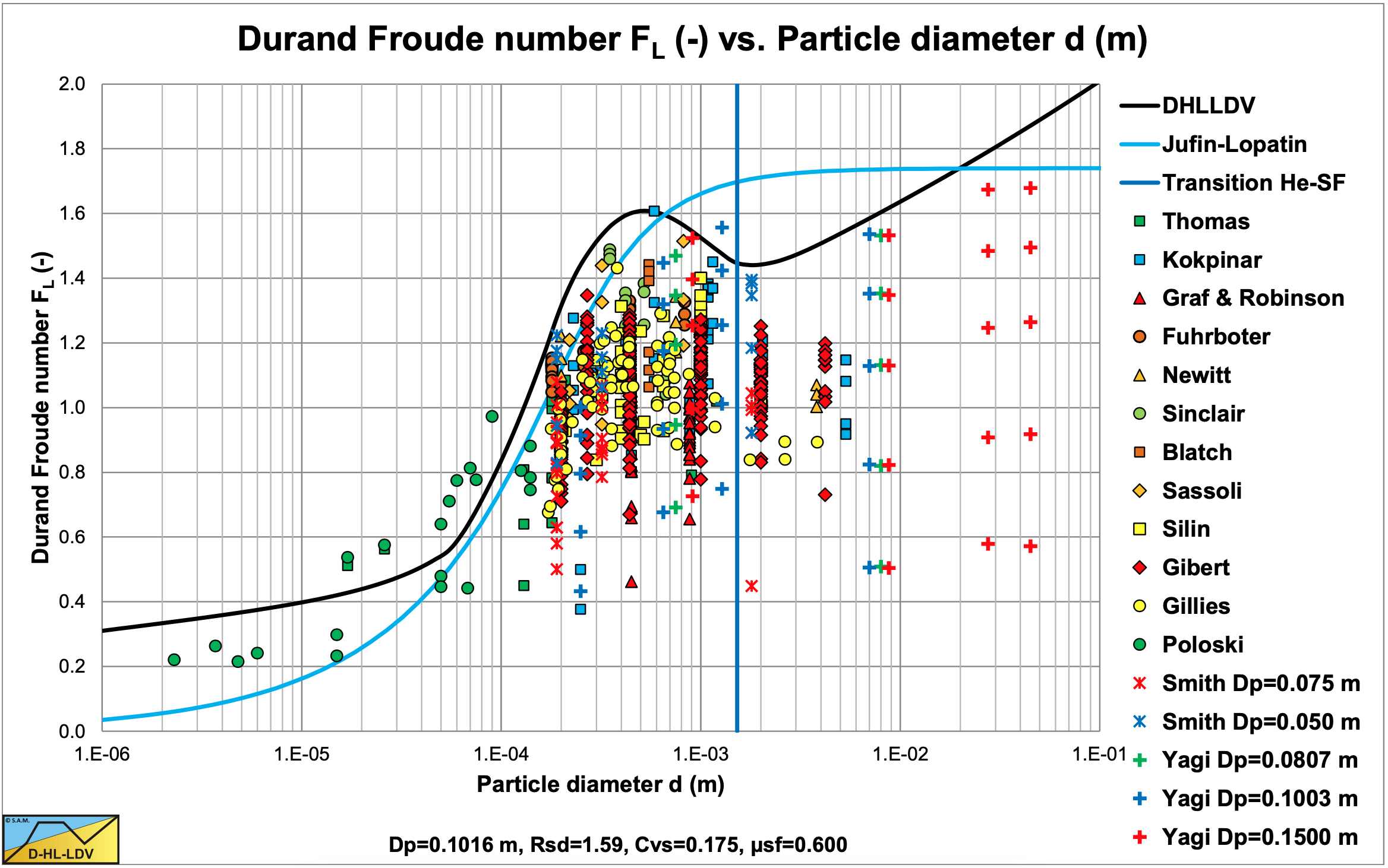
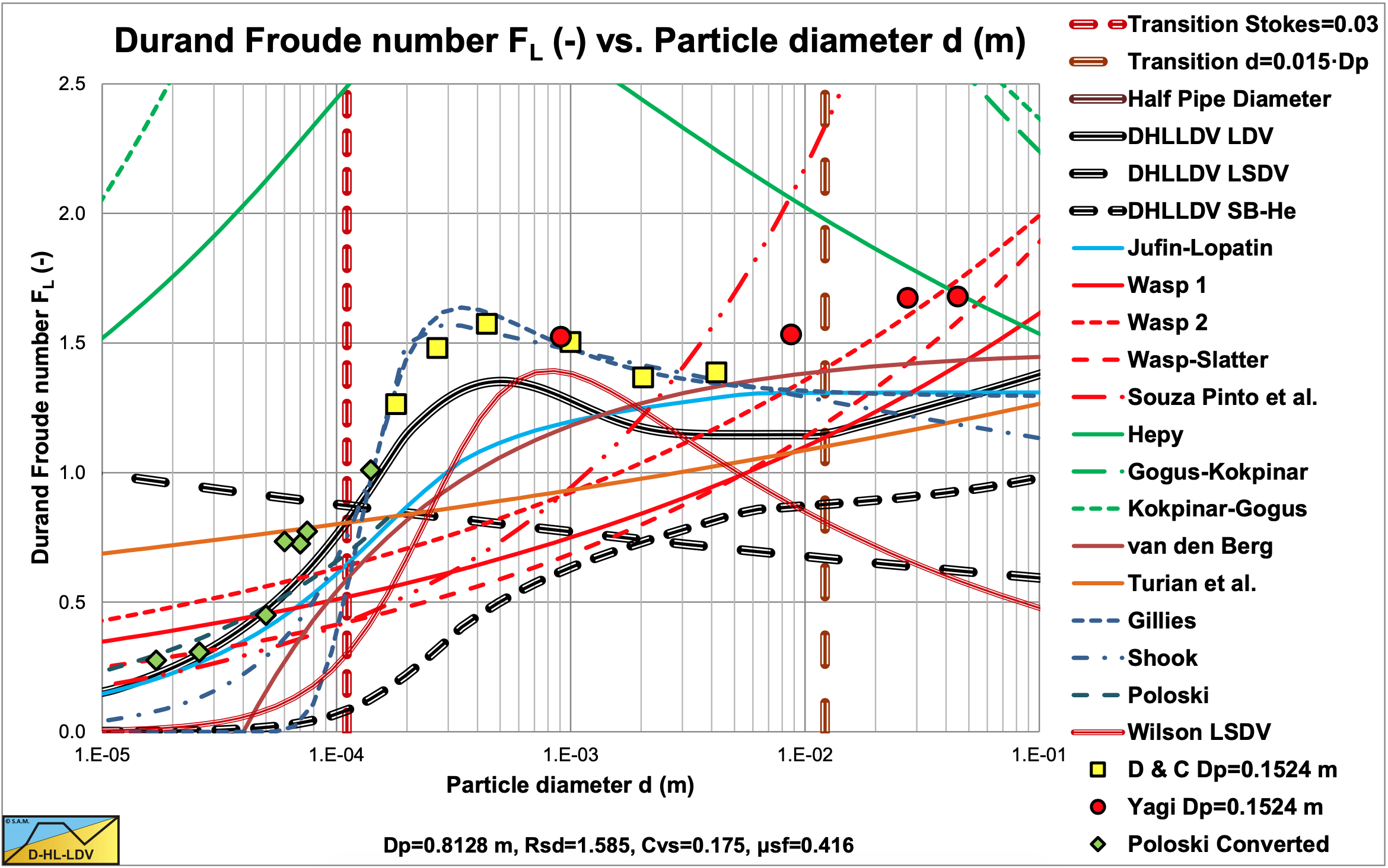
Figure 6.27-1 shows many data points of various authors for sand and gravel in water. Each column of data points shows the results of experiments with different volumetric concentrations, where the highest point were at volumetric concentrations of about 20%. The experimental data also showed that smaller pipe diameters, in general, give higher Durand & Condolios (1952) Froude FL numbers. The two curves in the graph are for the Jufin & Lopatin (1966) equation, which is only valid for sand and gravel, and the DHLLDV Framework which is described in chapter 7 of this book. Both models give a sort of upper limit to the LDV. The data points of the very small particle diameters, Thomas (1979), were carried out in a 0.0189 m pipe, while the graph is constructed for an 0.1016 (4 inch) pipe, resulting in a slightly lower curve. Based on the upper limit of the data points, the following is observed, from very small particles to very large particles (left to right in the graph):
- For very small particles, there seems to be a lower limit for the FL value.
- For small particles, the FL value increases to a maximum for a particle size of about d=0.5 mm.
- For medium sized particles with a particle size d>0.5 mm, the FL value decreases to a minimum for a particle size of about d=2 mm. Above 2 mm, the FL value will remain constant according to Durand & Condolios (1952).
- For particles with d/Dp>0.015, the Wilson et al. (1992) criterion for real suspension/saltation, the FL value increases again. This criterion is based on the ratio particle diameter to pipe diameter and will start at a large particle diameter with increasing pipe diameter.
Because there are numerous equations for the LDV, some based on physics, but most based on curve fitting, a selection is made of LDV equations and methods from literature. The results of these equations are discussed in the conclusions and discussion.
6.27.2 Wilson (1942)
Wilson (1942) used the minimum hydraulic gradient velocity (MHGV) for the LDV. This concept has been followed by many others, but has nothing to do with the physical LDV, only with the minimum power requirement. The model is based on the terminal settling velocity.
6.27.3 Durand & Condolios (1952)
Durand & Condolios (1952) derived a relatively simple equation based on the Froude number of the flow.
\[\ \mathrm{F}_{\mathrm{L}}=\frac{\mathrm{v}_{\mathrm{l s}, \mathrm{ld v}}}{\sqrt{\mathrm{2 \cdot g} \cdot \mathrm{R}_{\mathrm{s d}} \cdot \mathrm{D}_{\mathrm{p}}}}\]
For the value of the Froude number FL a graph is published, showing an increasing value up to a maximum of about 1.55 at a particle size of d=0.5 mm, after which FL decreases to an asymptotic value of about 1.34 for very large particles. The graph also shows a dependency of the LDV with respect to the volumetric concentration. The Froude number FL shows a maximum for volumetric concentrations between 15% and 20%. The FL value does not depend on the pipe diameter and the relative submerged density, only on the particle diameter and the volumetric concentration. It should be mentioned that there is a discrepancy of a factor Rsd1/2 between the graph published by Durand & Condolios (1952) and the graph published by Durand (1953), giving a factor of about 1.28. The graph as used by many authors overestimates the Durand Froude number by this factor. Figure 6.27-2, Figure 6.27-3, Figure 6.27-4 and Figure 6.27-5 show the correct and incorrect Durand Froude numbers compared with many other equations. Compared with data from many authors however, the wrong graph seems to be right with respect to the prediction of the LDV, which is probably the reason nobody found this mistake or made comments about it.
6.27.4 Newitt et al. (1955)
Newitt et al. (1955), like Wilson (1942), focused on the terminal settling velocity in their modeling. They did not really give an equation for the LDV, however they gave a relation for the transition between the sliding bed regime and the heterogeneous regime based on the terminal settling velocity, giving vSB-He=17·vt. This regime transition velocity may however be considered a lower limit to the LDV.
6.27.5 Jufin & Lopatin (1966)
Jufin & Lopatin (1966) defined the Limit Deposit Velocity as (sometimes a value of 8 is used instead of 8.3):
\[\ \mathrm{v}_{\mathrm{l s}, \mathrm{ldv}}=\mathrm{8 .3} \cdot\left(\mathrm{C}_{\mathrm{v t}} \cdot \Psi^{*}\right)^{1 / 6} \cdot \mathrm{D}_{\mathrm{p}}^{\mathrm{1 / 3}}\]
It is clear that this Limit Deposit Velocity also does not have the dimension of velocity, but the cube root of length. In dimensionless for giving:
\[\ \mathrm{ F_{L}=\frac{v_{l s, ld v}}{\left(2 \cdot g \cdot D_{p} \cdot R_{s d}\right)^{1 / 2}}}=9.23 \cdot \frac{\left(\mathrm{c_{v t}}\right)^{1 / 6} \cdot\left(\frac{\mathrm{v_{t}}}{\sqrt{\mathrm{g \cdot d}}}\right)^{1 / 4} \cdot\left(v_{\mathrm{l}} \cdot \mathrm{g}\right)^{1 / 9}}{\left(2 \cdot \mathrm{g \cdot D_{p} \cdot R_{s d}}\right)^{1 / 6}}\]
The Froude number FL decreases with increasing pipe diameter (power -1/6) and increases with increasing particle diameter. The FL value also decreases with increasing relative submerged density (power -1/6).
6.27.6 Zandi & Govatos (1967)
Zandi & Govatos (1967) defined a parameter N and stated that N<40 means saltating flow and N>40 heterogeneous flow. Apparently in their perception heterogeneous flow cannot contain saltation, which differs from the perception of others. The parameter N is:
\[\ \mathrm{N}=\frac{\mathrm{v}_{\mathrm{l} \mathrm{s}}^{\mathrm{2}} \cdot \sqrt{\mathrm{C}_{\mathrm{D}}}}{\mathrm{g} \cdot \mathrm{R}_{\mathrm{s d}} \cdot \mathrm{D}_{\mathrm{p}} \cdot \mathrm{C}_{\mathrm{v t}}}<\mathrm{4 0}\]
This gives for the Limit Deposit Velocity:
\[\ \mathrm{v}_{\mathrm{l s}, \mathrm{ld v}}=\sqrt{\frac{\mathrm{4 0 \cdot g \cdot R}_{\mathrm{s d}} \cdot \mathrm{D}_{\mathrm{p}} \cdot \mathrm{C}_{\mathrm{v t}}}{\sqrt{\mathrm{C}_{\mathrm{D}}}}}\]
In terms of the Durand & Condolios (1952) Froude number FL this gives:
\[\ \mathrm{ F_{L}=\frac{v_{l s, l d v}}{\sqrt{2 \cdot g \cdot R_{s d} \cdot D_{p}}}=\sqrt{\frac{20 \cdot C_{v t}}{\sqrt{C_{D}}}}}\]
From literature it is not clear whether Zandi & Govatos (1967) used the particle drag coefficient or the particle Froude number. In the perception of Zandi & Govatos (1967), the Froude number FL depends on the volumetric concentration and on the particle drag coefficient, which means a constant value for large particles.
6.27.7 Charles (1970)
Charles (1970) suggested to use the Minimum Hydraulic Gradient Velocity (MHGV) as an estimate for the Limit Deposit Velocity (LDV) since these are close. This MHGV can be obtained by differentiating the above equation with respect to the line speed vls. This gives:
\[\ \mathrm{i}_{\mathrm{m}}=\mathrm{i}_{\mathrm{l}} \cdot\left(\frac{\mathrm{K}}{\mathrm{R}_{\mathrm{s d}}} \cdot \Psi^{-1.5}+\mathrm{1}\right) \cdot \mathrm{C}_{\mathrm{v t}} \cdot \mathrm{R}_{\mathrm{s d}}+\mathrm{i}_{\mathrm{l}}\]
Or:
\[\ \begin{array}{left} \mathrm{i}_{\mathrm{m}}=\frac{\lambda_{\mathrm{l}} \cdot \mathrm{v}_{\mathrm{l s}}^{2}}{\mathrm{2} \cdot \mathrm{g} \cdot \mathrm{D}_{\mathrm{p}}} \cdot\left(\frac{\mathrm{K}}{\mathrm{R}_{\mathrm{s} \mathrm{d}}} \cdot\left(\left(\frac{\mathrm{v}_{\mathrm{l} \mathrm{s}}^{2}}{\mathrm{g} \cdot \mathrm{D}_{\mathrm{p}} \cdot \mathrm{R}_{\mathrm{s} \mathrm{d}}}\right) \cdot \sqrt{\mathrm{C}_{\mathrm{x}}}\right)^{-1.5}+\mathrm{1}\right) \cdot \mathrm{C}_{\mathrm{v} \mathrm{t}} \cdot \mathrm{R}_{\mathrm{s} \mathrm{d}}+\frac{\lambda_{\mathrm{l}} \cdot \mathrm{v}_{\mathrm{ls}}^{2}}{\mathrm{2} \cdot \mathrm{g} \cdot \mathrm{D}_{\mathrm{p}}}\\
\mathrm{i}_{\mathrm{m}}=\frac{\lambda_{\mathrm{l}}}{\mathrm{2} \cdot \mathrm{g} \cdot \mathrm{D}_{\mathrm{p}}} \left(\cdot\left(\mathrm{1}+\mathrm{C}_{\mathrm{v} \mathrm{t}} \cdot \mathrm{R}_{\mathrm{s d}}\right) \cdot \mathrm{v}_{\mathrm{l} \mathrm{s}}^{2}+\left(\mathrm{K} \cdot\left(\frac{\mathrm{g} \cdot \mathrm{D}_{\mathrm{p}} \cdot \mathrm{R}_{\mathrm{s} \mathrm{d}}}{\sqrt{\mathrm{C}_{\mathrm{x}}}}\right)^{1.5} \cdot \mathrm{C}_{\mathrm{v} \mathrm{t}}\right) \cdot \frac{\mathrm{1}}{\mathrm{v}_{\mathrm{l s}}}\right)\end{array}\]
This gives for the MHGV:
\[\ \mathrm{v}_{\mathrm{ls}, \mathrm{M H G V}}=\left(\frac{\left(\mathrm{K} \cdot\left(\frac{\mathrm{g} \cdot \mathrm{D}_{\mathrm{p}} \cdot \mathrm{R}_{\mathrm{s} \mathrm{d}}}{\sqrt{\mathrm{C}_{\mathrm{x}}}}\right)^{1.5} \cdot \mathrm{C}_{\mathrm{v} \mathrm{t}}\right)}{\mathrm{2} \cdot\left(\mathrm{1}+\mathrm{C}_{\mathrm{v} \mathrm{t}} \cdot \mathrm{R}_{\mathrm{s d}}\right)}\right)^{1 / 3}\]
6.27.8 Graf et al. (1970) & Robinson (1971)
Graf et al. (1970) & Robinson (1971) carried out experiments at low concentrations in pipes with small positive and negative inclination angles. They added the inclination angle to the Durand Froude number FL.
Assuming the concentration was the only important parameter, the following fit function was found:
\[\ \mathrm{F}_{\mathrm{L}}=\frac{\mathrm{v}_{\mathrm{l} \mathrm{s}, \mathrm{l} \mathrm{d} \mathrm{v}}}{\sqrt{\mathrm{2} \cdot \mathrm{g} \cdot \mathrm{D}_{\mathrm{p}} \cdot \mathrm{R}_{\mathrm{s d}}}} \cdot(\mathrm{1}-\tan (\theta))=\mathrm{0} . \mathrm{9 0 1} \cdot \mathrm{C}_{\mathrm{v}}^{\mathrm{0.106}}\]
Including the particle diameter in the correlation, the following equation was found:
\[\ \mathrm{F_{\mathrm{L}}=\frac{v_{\mathrm{ls}, \mathrm{ldv}}}{\sqrt{2 \cdot \mathrm{g} \cdot \mathrm{D}_{\mathrm{p}} \cdot \mathrm{R}_{\mathrm{sd}}}} \cdot(1-\tan (\theta))=0.928 \cdot \mathrm{C}_{\mathrm{v}}^{0.105}} \cdot \mathrm{d^{0.058}}\]
6.27.9 Wilson & Judge (1976)
The Wilson & Judge (1976) correlation is used for particles for which the Archimedes number is less than about 80. The correlation is expressed in terms of the Durand Froude number FL according to:
\[\ \mathrm{F}_{\mathrm{L}}=\frac{\mathrm{v}_{\mathrm{l s}, \mathrm{ld} \mathrm{v}}}{\sqrt{\mathrm{2} \cdot \mathrm{g} \cdot \mathrm{D}_{\mathrm{p}} \cdot \mathrm{R}_{\mathrm{s d}}}}=\left(2+\mathrm{0 . 3} \cdot \log _{10}\left(\frac{\mathrm{d}}{\mathrm{D}_{\mathrm{p}} \cdot \mathrm{C}_{\mathrm{D}}}\right)\right)\]
This gives for the Limit Deposit Velocity:
\[\ \mathrm{v}_{\mathrm{l s}, \mathrm{ld v}}=\left(\mathrm{2}+\mathrm{0 .3} \cdot \log _{\mathrm{1 0}}\left(\frac{\mathrm{d}}{\mathrm{D}_{\mathrm{p}} \cdot \mathrm{C}_{\mathrm{D}}}\right)\right) \cdot \sqrt{\mathrm{2 \cdot g \cdot \mathrm { D } _ { \mathrm { p } }} \cdot \mathrm{R}_{\mathrm{s d}}}\]
The applicability is approximately where the dimensionless group in the logarithm is larger than 10-5 .
6.27.10 Wasp et al. (1977)
Wasp et al. (1977) derived an equation similar to the Durand & Condolios (1952) equation, but instead of using a graph for the Froude number FL, they quantified the influence of the concentration and the particle diameter to pipe diameter ratio. It should be noted that there are several almost similar equations found in literature where the powers of the volumetric concentration and the proportionality coefficient may differ slightly.
\[\ \begin{array}{left} \mathrm{v}_{\mathrm{l s}, \mathrm{l d v}}=\mathrm{4} \cdot \mathrm{C}_{\mathrm{v s}}^{1/5} \cdot \sqrt{\mathrm{2} \cdot \mathrm{g} \cdot \mathrm{D}_{\mathrm{p}} \cdot \mathrm{R}_{\mathrm{s d}}} \cdot\left(\frac{\mathrm{d}}{\mathrm{D}_{\mathrm{p}}}\right)^{1 / 6}=\mathrm{F}_{\mathrm{L}} \cdot \sqrt{\mathrm{2} \cdot \mathrm{g} \cdot \mathrm{D}_{\mathrm{p}} \cdot \mathrm{R}_{\mathrm{s d}}}\\
\mathrm{F}_{\mathrm{L}}=\frac{\mathrm{v}_{\mathrm{l} \mathrm{s}, \mathrm{ld} \mathrm{v}}}{\sqrt{\mathrm{2} \cdot \mathrm{g} \cdot \mathrm{D}_{\mathrm{p}} \cdot \mathrm{R}_{\mathrm{s d}}}}=\mathrm{4} \cdot \mathrm{C}_{\mathrm{v s}}^{1 / 5} \cdot\left(\frac{\mathrm{d}}{\mathrm{D}_{\mathrm{p}}}\right)^{1 / 6}\end{array}\]
The Froude number FL decreases slightly with increasing pipe diameter and increases slightly with increasing particle diameter. The increase of FL with increasing volumetric concentration, without finding a maximum, is probably due to the fact that the volumetric concentrations were hardly higher than 20%.
The equations are also found in literature with slightly different coefficients for the volumetric concentration and the proportionality constant. The behavior however is the same. With an equation of this type never a maximum LDV for particle diameters close to 0.5 mm can be found, since the equations give a continues increase of the LDV with increasing particle diameter.
\[\ \begin{array}{left} \mathrm{v}_{\mathrm{ls}, \mathrm{ldv}}=3.8 \cdot \mathrm{C}_{\mathrm{vs}}^{0.25} \cdot \sqrt{2 \cdot \mathrm{g} \cdot \mathrm{D}_{\mathrm{p}} \cdot \mathrm{R}_{\mathrm{sd}}} \cdot\left(\frac{\mathrm{d}}{\mathrm{D}_{\mathrm{p}}}\right)^{1 / 6}=\mathrm{F}_{\mathrm{L}} \cdot \sqrt{2 \cdot \mathrm{g} \cdot \mathrm{D}_{\mathrm{p}} \cdot \mathrm{R}_{\mathrm{sd}}}\\
\mathrm{F}_{\mathrm{L}}=\frac{\mathrm{v}_{\mathrm{ls}, \mathrm{ldv}}}{\sqrt{2 \cdot \mathrm{g} \cdot \mathrm{D}_{\mathrm{p}} \cdot \mathrm{R}_{\mathrm{sd}}}}=3.8 \cdot \mathrm{C}_{\mathrm{vs}}^{0.25} \cdot\left(\frac{\mathrm{d}}{\mathrm{D}_{\mathrm{p}}}\right)^{1 / 6}\end{array}\]
6.27.11 Thomas (1979)
Thomas (1979) derived an equation for very small particles, proving that there is a lower limit to the LDV. The method is based on the fact that particles smaller than the thickness of the viscous sub layer will be in suspension due to turbulent eddies in the turbulent layer, but may still settle in the laminar viscous sub layer. By using a force balance on a very thin bed layer in the viscous sub layer, he found the following equation:
\[\ \mathrm{v}_{\mathrm{ls}, \mathrm{ldv}}=1.49 \cdot\left(\mathrm{g} \cdot \mathrm{R}_{\mathrm{sd}} \cdot \mathrm{C}_{\mathrm{vb}} \cdot v_{\mathrm{l}} \cdot \mu_{\mathrm{sf}}\right)^{1 / 3} \cdot \sqrt{\frac{\mathrm{8}}{\lambda_{\mathrm{l}}}}\]
\[\ \mathrm{F}_{\mathrm{L}}=\frac{\mathrm{v}_{\mathrm{l s}, \mathrm{ld v}}}{\sqrt{\mathrm{2} \cdot \mathrm{g} \cdot \mathrm{D}_{\mathrm{p}} \cdot \mathrm{R}_{\mathrm{s d}}}}=\frac{\mathrm{1 . 4 9 \cdot ( \mathrm { g } \cdot \mathrm { R } _ { \mathrm { s d } } \cdot \mathrm { C } _ { \mathrm { v b } }}{ \cdot v_ { \mathrm { l } } \cdot \mathrm { \mu } _ { \mathrm { s f } } ) ^ { 1 / 3 }} \cdot \sqrt{\frac{\mathrm{8}}{\lambda_{\mathrm{l}}}}}{\sqrt{\mathrm{2 \cdot \mathrm { g } \cdot \mathrm { D } _ { \mathrm { p } } \cdot \mathrm { R } _ { \mathrm { s d } }}}}\]
The Froude number FL does not depend on the particle size, but on the thickness of the viscous sub layer and so on the Darcy Weisbach friction coefficient. The Froude number FL does depend on the pipe diameter to a power of about -0.4, due to the Darcy Weisbach friction factor. The line speed found by Thomas (1979) is however an LSDV and not the LDV, so the LDV may be expected to have a higher value. Thomas (1979) also found that the relation between the LDV and the pipe diameter has a dependency with a power between 0.1 as a lower limit and 0.5 as an upper limit.
6.27.12 Oroskar & Turian (1980)
Oroskar & Turian (1980) derived an equation based on balancing the energy required to suspend the particles with the energy derived from the dissipation of an appropriate fraction of the turbulent eddies.
\[\ \mathrm{\frac{v_{\mathrm{ls}, \mathrm{ldv}}}{\sqrt{\mathrm{g} \cdot \mathrm{d} \cdot \mathrm{R}_{\mathrm{sd}}}}}=\left(5 \cdot \mathrm{C}_{\mathrm{vs}} \cdot\left(1-\mathrm{C}_{\mathrm{vs}}\right)^{2 \cdot \beta-1} \cdot\left(\frac{\mathrm{D}_{\mathrm{p}}}{\mathrm{d}}\right) \cdot\left(\frac{\mathrm{D}_{\mathrm{p}} \cdot \sqrt{\mathrm{g} \cdot \mathrm{d} \cdot \mathrm{R}_{\mathrm{sd}}}}{v_{\mathrm{l}}}\right)^{1 / 8}\right)^{8 / 15}\]
In terms of the Froude number FL this gives:
\[\ \begin{array}{left} \mathrm{F}_{\mathrm{L}} &=\frac{\mathrm{v}_{\mathrm{l} \mathrm{s}, \mathrm{ld} \mathrm{v}}}{\sqrt{\mathrm{2 \cdot \mathrm { g } \cdot \mathrm { R } _ { \mathrm { s d } } \cdot \mathrm { D } _ { \mathrm { p } }}}} \\ &=\left(\mathrm{5} \cdot \mathrm{C}_{\mathrm{v s}} \cdot\left(\mathrm{1 - C}_{\mathrm{v s}}\right)^{2 \cdot \beta-1} \cdot\left(\frac{\mathrm{D}_{\mathrm{p}}}{\mathrm{d}}\right) \cdot\left(\frac{\mathrm{D}_{\mathrm{p}} \cdot \sqrt{\mathrm{g} \cdot \mathrm{d} \cdot \mathrm{R}_{\mathrm{s d}}}}{v_{\mathrm{l}}}\right)^{1 / 8}\right)^{8 / 1 \mathrm{5}} \cdot \frac{\sqrt{\mathrm{g} \cdot \mathrm{d} \cdot \mathrm{R}_{\mathrm{s d}}}}{\sqrt{\mathrm{2 \cdot \mathrm { g } \cdot \mathrm { R } _ { \mathrm { s d } } \cdot \mathrm { D } _ { \mathrm { p } }}}} \end{array}\]
The Froude number FL shows a maximum somewhere near 15%-20% depending on the particle diameter. The FL value increases slightly with an increasing pipe diameter (power 1/10). The FL value does not depend directly on the particle diameter. The FL value depends very slightly on the relative submerged density (power 1/30). Oroskar & Turian (1980) also published an empirical equation based on many experiments.
\[\ \frac{\mathrm{v}_{\mathrm{l s}, \mathrm{ld v}}}{\sqrt{\mathrm{g} \cdot \mathrm{d} \cdot \mathrm{R}_{\mathrm{s d}}}}=\mathrm{1 .85} \cdot \mathrm{C _ { \mathrm { v s } }}^{\mathrm{0 .1536}} \cdot\left(\mathrm{1 - C}_{\mathrm{v s}}\right)^{\mathrm{0 . 3 5 6 4}} \cdot\left(\frac{\mathrm{D _ { \mathrm { p } }}}{\mathrm{d}}\right)^{\mathrm{0 . 3 7 8}} \cdot\left(\frac{\mathrm{D _ { p }} \cdot \sqrt{\mathrm{g} \cdot \mathrm{d \cdot R}_{\mathrm{s d}}}}{v_{\mathrm{l}}}\right)^{0.09}\]
In terms of the Froude number FL this gives:
\[\ \begin{array}{left} \mathrm{F}_{\mathrm{L}} &=\frac{\mathrm{v}_{\mathrm{l} \mathrm{s}, \mathrm{ld} \mathrm{v}}}{\sqrt{\mathrm{2} \cdot \mathrm{g} \cdot \mathrm{R}_{\mathrm{s d}} \cdot \mathrm{D}_{\mathrm{p}}}} \\
&=\mathrm{1 .85} \cdot \mathrm{C}_{\mathrm{v s}}^{0.1536} \cdot\left(1-\mathrm{C}_{\mathrm{v} \mathrm{s}}\right)^{0.3564} \cdot\left(\frac{\mathrm{D}_{\mathrm{p}}}{\mathrm{d}}\right)^{0.378} \cdot\left(\frac{\mathrm{D}_{\mathrm{p}} \cdot \sqrt{\mathrm{g} \cdot \mathrm{d} \cdot \mathrm{R}_{\mathrm{s d}}}}{v_{\mathrm{l}}}\right)^{0.09} \cdot \frac{\sqrt{\mathrm{g} \cdot \mathrm{d} \cdot \mathrm{R}_{\mathrm{s d}}}}{\sqrt{\mathrm{2 \cdot g} \cdot \mathrm{R}_{\mathrm{s d}} \cdot \mathrm{D}_{\mathrm{p}}}} \end{array}\]
The Froude number FL shows a maximum somewhere near 15%-20% concentration depending on the particle diameter. The FL value decreases very slightly with increasing pipe diameter (power -0.032). The FL value increases slightly with increasing particle diameter (power 0.167). The FL value increases slightly with an increasing relative submerged density (power 0.045).
In the comparison of Oroskar & Turian (1980), the empirical equation gives less deviation compared to the theoretical equation. The main difference between the two equations is the dependency of the FL value on the pipe diameter (+0.1 versus -0.032).
6.27.13 Parzonka et al. (1981)
Parzonka et al. (1981) investigated to influence of the spatial volumetric concentration on the LDV. The data obtained from literature covered a wide range of pipe diameters, from 0.0127 m to 0.8000 m. The particles were divided into 5 categories:
- Small size sand particles ranging from 0.1 mm to 0.28 mm.
- Medium and coarse size sand particles ranging from 0.4 mm to 0.85 mm.
- Coarse size sand and gravel ranging from 1.15 mm to 19 mm.
- Small size high density materials ranging from 0.005 mm to 0.3 mm.
- Coal particles ranging from 1 mm to 2.26 mm.
Their conclusion state that the spatial concentration has a large influence on the LDV. The increase of the LDV with increasing concentration was already recognized before, but the occurrence of a maximum LDV at a concentration of about 15% and a decrease of the LDV with further increasing concentration was not commonly noted. Parzonka et al. (1981) also concluded that the presence of very small particles in the PSD reduces the LDV. It should be noted that Parzonka et al. (1981) collected a lot of valuable data.
6.27.14 Turian et al. (1987)
Turian et al. (1987) improves the relation of Oroskar & Turian (1980), based on more experiments, giving:
\[\ \mathrm{v}_{\mathrm{ls}, \mathrm{ldv}}= \mathrm{1 . 7 9 5 1 \cdot \mathrm { C } _ { \mathrm { v s } } ^ { 0 . 1 0 8 7 }} \cdot\left(\mathrm{1 - C}_{\mathrm{v s}}\right)^{0.2501} \cdot\left(\frac{\mathrm{D}_{\mathrm{p}} \cdot \sqrt{\mathrm{g} \cdot \mathrm{D}_{\mathrm{p}} \cdot \mathrm{R}_{\mathrm{s d}}}}{v_{\mathrm{l}}}\right)^{0.00179} \cdot\left(\frac{\mathrm{d}}{\mathrm{D}_{\mathrm{p}}}\right)^{0.06623} \cdot \sqrt{\mathrm{2 . g} \cdot \mathrm{R}_{\mathrm{s d}} \cdot \mathrm{D}_{\mathrm{p}}}\]
In terms of the Froude number FL this gives:
\[\ \begin{array}{left} \mathrm{F}_{\mathrm{L}} &=\frac{\mathrm{v}_{\mathrm{l s}, \mathrm{ld v}}}{\sqrt{\mathrm{2} \cdot \mathrm{g} \cdot \mathrm{R}_{\mathrm{s d}} \cdot \mathrm{D}_{\mathrm{p}}}} \\ &=\mathrm{1 . 7 9 5 1 \cdot \mathrm { C } _ { \mathrm { v } \mathrm { s } } ^ { 0 . 1 0 8 7 } \cdot ( 1 - \mathrm { C } _ { \mathrm { v s } } ) ^ { 0 . 2 5 0 1 } \cdot \left( \frac { \mathrm { D } _ { \mathrm { p } } \cdot \sqrt { \mathrm { g } \cdot \mathrm { D } _ { \mathrm { p } } \cdot \mathrm { R } _ { \mathrm { s } \mathrm { d } } }}{ { v _ { \mathrm { l } } } } \right) ^ { 0 . 0 0 1 7 9 }} \cdot\left(\frac{\mathrm{d}}{\mathrm{D}_{\mathrm{p}}}\right)^{0.0662 \mathrm{3}} \end{array}\]
The Froude number FL shows a maximum somewhere near 15%-20% concentration depending on the particle diameter. The Froude number FL increases slightly with increasing particle diameter. The Froude number FL decreases slightly with increasing pipe diameter with a power of -0.0635.
6.27.15 Davies (1987)
Davies (1987) based the LDV on the equilibrium between the gravity force and the eddy velocity pressure force. Only eddies with a size close to the particle diameter can lift the particles. Much smaller eddies are not strong enough and will be involved in viscous dissipation, while much larger eddies cannot closely approach the bottom of the pipe where the solids are sedimented. The downward directed force, the sedimentation force, caused by the difference in density between the particle and the water can be calculated by:
\[\ \mathrm{F_{\text {down }}=\left(\rho_{\mathrm{s}}-\rho_{\mathrm{l}}\right) \cdot \mathrm{g} \cdot \frac{\pi}{6} \cdot \mathrm{d}^{3} \cdot\left(1-\mathrm{C}_{\mathrm{vs}}\right)^{\mathrm{n}}}\]
Where n depends on the Reynolds number related to the terminal settling velocity. The eddy fluctuation force equals the eddy pressure times the area of the particle, giving:
\[\ \mathrm{F_{u p}=\rho_{l} \cdot \frac{\pi}{4} \cdot d^{2} \cdot v_{e f}^{2}}\]
Where vef is the turbulent fluctuation velocity for the eddies concerned. When no particles are settling on the bottom of the pipe, so all the particles are just being lifted by the eddies, this results in a turbulent fluctuation velocity:
\[\ \mathrm{v}_{\mathrm{ef}}=\sqrt{\frac{2}{3} \cdot \mathrm{g} \cdot \mathrm{R}_{\mathrm{sd}} \cdot \mathrm{d} \cdot\left(1-\mathrm{C}_{\mathrm{v s}}\right)^{\mathrm{n}}}\]
The last step is to relate the turbulent fluctuation velocity to the LDV. The turbulent fluctuation velocity is related to the power dissipated per unit mass of fluid by:
\[\ \mathrm{v}_{\mathrm{ef}}^{\mathrm{3}}=\mathrm{P} \cdot \mathrm{d} \quad\text{ with: }\quad \mathrm{P}=\lambda_{\mathrm{l}} \cdot \frac{\mathrm{v}_{\mathrm{ls,ldv}}^3 }{\mathrm{2} \cdot \mathrm{D}_{\mathrm{p}}}\]
Using an approximation for the Darcy Weisbach friction factor according to Blasius:
\[\ \lambda_{\mathrm{l}}=\frac{\mathrm{0 . 3 1 6 4}}{\mathrm{R e}^{\mathrm{1 / 4}}} \approx \mathrm{0 . 3 2} \cdot v_{\mathrm{l}}^{\mathrm{0 . 2 5}} \cdot \mathrm{v}_{\mathrm{l s}}^{-\mathrm{0 . 2 5}} \cdot \mathrm{D}_{\mathrm{p}}^{-\mathrm{0 . 2 5}}\]
Gives:
\[\ \mathrm{v}_{\mathrm{ef}}=\left(0.16 \cdot v_{\mathrm{l}}^{0.25} \cdot \mathrm{v}_{\mathrm{ls}, \mathrm{ldv}}^{2.75} \cdot \mathrm{D}_{\mathrm{p}}^{-1.25} \cdot \mathrm{d}\right)^{1 / 3} \quad\text{ or }\quad \mathrm{v}_{\mathrm{ef}}=\left(\lambda_{\mathrm{l}} \cdot \frac{\mathrm{v}_{\mathrm{ls}, \mathrm{ldv}}^{3}}{2 \cdot \mathrm{D}_{\mathrm{p}}} \cdot \mathrm{d}\right)^{1 / 3}\]
The eddy velocity is corrected for the presence of particles by:
\[\ \begin{array}{left} \mathrm{v}_{\mathrm{e f}} \cdot\left(\mathrm{1}+\mathrm{\alpha} \cdot \mathrm{C}_{\mathrm{v s}}\right)=\left(\mathrm{0 . 1 6} \cdot v_{\mathrm{l}}^{\mathrm{0} . \mathrm{2 5}} \cdot \mathrm{v}_{\mathrm{l} \mathrm{s}, \mathrm{ld} \mathrm{v}}^{\mathrm{2 . 7 5}} \cdot \mathrm{D}_{\mathrm{p}}^{-\mathrm{1 . 2 5}} \cdot \mathrm{d}\right)^{\mathrm{1 / 3}}\\
\text { Or}\\
\mathrm{v}_{\mathrm{ef}} \cdot\left(1+\alpha \cdot \mathrm{C}_{\mathrm{vs}}\right)=\left(\lambda_{\mathrm{l}} \cdot \frac{\mathrm{v}_{\mathrm{l s}, \mathrm{ldv}}^{3}}{2 \cdot \mathrm{D}_{\mathrm{p}}} \cdot \mathrm{d}\right)^{1 / 3}\end{array}\]
Now equating the sedimentation velocity and the eddy velocity gives:
\[\ \frac{\left(0.16 \cdot v_{\mathrm{l}}^{0.25} \cdot \mathrm{v_{ls, ldv}}^{2.75} \cdot \mathrm{D_{p}^{-1.25}} \cdot \mathrm{d}\right)^{1 / 3}}{\left(1+\alpha \cdot \mathrm{C_{v s}}\right)}=\sqrt{\frac{2}{3} \cdot \mathrm{g \cdot R_{s d} \cdot d \cdot\left(1-C_{v s}\right)^{n}}}\]
Or:
\[\ \frac{\left(\lambda_{\mathrm{l}} \cdot \frac{\mathrm{v}_{\mathrm{ls}, \mathrm{ldv}}^{3}}{2 \cdot \mathrm{D}_{\mathrm{p}}} \cdot \mathrm{d}\right)^{1 / 3}}{\left(1+\alpha \cdot \mathrm{C}_{\mathrm{vs}}\right)}=\sqrt{\frac{2}{3} \cdot \mathrm{g} \cdot \mathrm{R}_{\mathrm{sd}} \cdot \mathrm{d} \cdot\left(1-\mathrm{C}_{\mathrm{vs}}\right)^{\mathrm{n}}}\]
Giving:
\[\ \begin{array}{left} \mathrm{v}_{\mathrm{l s}, \mathrm{ld v}}=\mathrm{1 . 0 6 6} \cdot\left(\mathrm{1}+\mathrm{\alpha} \cdot \mathrm{C}_{\mathrm{v s}}\right)^{\mathrm{1} .091} \cdot\left(\mathrm{1}-\mathrm{C}_{\mathrm{v s}}\right)^{0.545 \cdot \mathrm{n}} \cdot v_{\mathrm{l}}^{-\mathrm{0} .091} \cdot \mathrm{d}^{0.181} \cdot\left(\mathrm{2} \cdot \mathrm{g} \cdot \mathrm{R}_{\mathrm{s d}}\right)^{0.545} \cdot \mathrm{D}_{\mathrm{p}}^{0.455}\\
\text{Or : }\\
\mathrm{v}_{\mathrm{l s}, \mathrm{ldv}}=\mathrm{0 . 7 2 7} \cdot\left(\frac{\mathrm{1}}{\lambda_{\mathrm{l}}}\right)^{1 / 3} \cdot\left(\frac{\mathrm{d}}{\mathrm{D}_{\mathrm{p}}}\right)^{1 / 6} \cdot\left(1+\alpha \cdot \mathrm{C}_{\mathrm{v s}}\right) \cdot\left(1-\mathrm{C}_{\mathrm{v s}}\right)^{1 / 2 \cdot \mathrm{n}} \cdot\left(2 \cdot \mathrm{g} \cdot \mathrm{R}_{\mathrm{s d}} \cdot \mathrm{D}_{\mathrm{p}}\right)^{1 / 2}\end{array}\]
The Durand Froude number is now:
\[\ \begin{array}{left}\mathrm{F}_{\mathrm{L}}=\frac{\mathrm{v}_{\mathrm{l s}, \mathrm{ldv}}}{\sqrt{\mathrm{2 \cdot g} \cdot \mathrm{D}_{\mathrm{p}} \cdot \mathrm{R}_{\mathrm{s d}}}}=\mathrm{1 . 0 6 6} \cdot\left(\mathrm{1}+\mathrm{\alpha} \cdot \mathrm{C}_{\mathrm{v s}}\right)^{\mathrm{1 . 0 9 1}} \cdot\left(\mathrm{1 - C}_{\mathrm{v s}}\right)^{0.545 \cdot \mathrm{n}} \cdot v_{\mathrm{l}}^{-\mathrm{0 . 0 9 1}} \cdot \mathrm{d}^{0.181} \cdot\left(\frac{\mathrm{2 \cdot g \cdot R}_{\mathrm{s d}}}{\mathrm{D}_{\mathrm{p}}}\right)^{0.045}\\
\text{Or : }\\
\mathrm{F}_{\mathrm{L}}=\frac{\mathrm{v}_{\mathrm{l s}, \mathrm{ld} \mathrm{v}}}{\sqrt{\mathrm{2} \cdot \mathrm{g} \cdot \mathrm{D}_{\mathrm{p}} \cdot \mathrm{R}_{\mathrm{s d}}}}=\mathrm{0 . 7 2 7} \cdot\left(\frac{\mathrm{1}}{\lambda_{\mathrm{l}}}\right)^{1 / 3} \cdot\left(\frac{\mathrm{d}}{\mathrm{D}_{\mathrm{p}}}\right)^{1 / 6} \cdot\left(1+\alpha \cdot \mathrm{C}_{\mathrm{v s}}\right) \cdot\left(1-\mathrm{C}_{\mathrm{v s}}\right)^{1 / 2 \cdot \mathrm{n}}\end{array}\]
The resulting equation gives a maximum Durand Froude number near a concentration of 15%. The factor α=3.64 according to Davies (1987). The equations containing the Darcy Weisbach friction factors were not reported by Davies (1987), but they give a better understanding. In fact the approximation used by Davies (1987) for the Darcy Weisbach friction factor is appropriate for small Reynolds numbers, but not for large Reynolds numbers as occur in dredging operations. The Durand Froude number decreases with the pipe diameter to a power depending on the Reynolds number, due to the Darcy Weisbach friction factor. Davies (1987) found a power of -0.045, but at larger Reynolds numbers this may approach -0.1.
6.27.16 Schiller & Herbich (1991)
Schiller & Herbich (1991) proposed an equation for the Durand & Condolios (1952) Froude number.
\[\ \mathrm{F_{L}}=\frac{\mathrm{v_{l s, ld v}}}{\sqrt{\mathrm{2 \cdot g \cdot D_{p} \cdot R_{s d}}}}=\mathrm{1.3 \cdot C_{v s}^{0.125}} \cdot\left(\mathrm{1-e^{-6.9 \cdot d_{50}}}\right)\]
The particle diameter in this equation is in mm. The equation is just a fit function on the Durand & Condolios (1952) data and has no physical meaning.
6.27.17 Gogus & Kokpinar (1993)
Gogus & Kokpinar (1993) proposed the following equation based on curve fitting:
\[\ \mathrm{v}_{\mathrm{l s}, \mathrm{ld v}}=\mathrm{0 . 1 2 4} \cdot\left(\frac{\mathrm{D _ { p }}}{\mathrm{d}}\right)^{0.537} \cdot \mathrm{C}_{\mathrm{v s}}^{\mathrm{0 . 3 2 2}} \cdot \mathrm{R}_{\mathrm{s d}}^{0.121} \cdot\left(\frac{\mathrm{v}_{\mathrm{t}} \cdot \mathrm{d}}{v_{\mathrm{l}}}\right)^{0.243} \cdot \sqrt{\mathrm{g} \cdot \mathrm{D}_{\mathrm{p}}}\]
With the Froude number FL:
\[\ \mathrm{F_{\mathrm{L}}}=\frac{\mathrm{v}_{\mathrm{ls}, \mathrm{ldv}}}{\sqrt{2 \cdot \mathrm{g} \cdot \mathrm{D}_{\mathrm{p}} \cdot \mathrm{R}_{\mathrm{sd}}}}=0.088 \cdot\left(\frac{\mathrm{D}_{\mathrm{p}}}{\mathrm{d}}\right)^{0.537} \cdot \mathrm{C}_{\mathrm{vs}}^{0.322} \cdot \mathrm{R}_{\mathrm{sd}}^{-0.379} \cdot\left(\frac{\mathrm{v}_{\mathrm{t}} \cdot \mathrm{d}}{v_{\mathrm{l}}}\right)^{0.243}\]
The Froude number FL depends strongly on the pipe diameter. An increasing pipe diameter results in an increasing FL. The FL value decreases with increasing relative submerged density. The influence of the particle diameter is more complex. First the FL value increases up to a particle diameter of 0.5 mm, for larger particles the FL value decreases, so there is a maximum near d=0.5 mm.
6.27.18 Gillies (1993)
Gillies (1993) derived an expression for the Durand & Condolios (1952) Froude number FL, giving a Limit Deposit Velocity of:
\[\ \mathrm{v}_{\mathrm{l s}, \mathrm{l d v}}=\mathrm{e}^{\left(\mathrm{0 . 5 1 - 0 . 0 0 7 3 \cdot C _ { \mathrm { D } } - \mathrm { 1 2 . 5 }} \cdot\left(\frac{(\mathrm{g} \cdot {v _ { \mathrm{l} }})^{2 / 3}}{\mathrm{g \cdot d}}-\mathrm{0 . 1 4}\right)^{2}\right)} \cdot \sqrt{\mathrm{2 \cdot g \cdot \mathrm { D } _ { \mathrm { p } } \cdot \mathrm { R } _ { \mathrm { s d } }}}\]
With the Froude number FL:
\[\ \mathrm{F}_{\mathrm{L}}=\frac{\mathrm{v}_{\mathrm{l s}, \mathrm{ld v}}}{\sqrt{\mathrm{2} \cdot \mathrm{g} \cdot \mathrm{D}_{\mathrm{p}} \cdot \mathrm{R}_{\mathrm{s d}}}}=\mathrm{e}^{\left({\mathrm{0 . 5 1 - 0 . 0 0 7 3} \cdot \mathrm{ C} _ { \mathrm { D } } - 1 2 . 5 \cdot \left( \frac { ( \mathrm { g } \cdot v _ { \mathrm{l} } ) ^ { 2 / 3 } } { \mathrm { g } \cdot \mathrm { d } } - \mathrm { 0 . 1 4 } \right) ^ { 2 }}\right)}\]
The Durand & Condolios (1952) Froude number FL does not depend on the pipe diameter and the volumetric concentration. The Froude number FL should be considered the maximum FL at a concentration near 20%. The FL value increases with the particle diameter to a maximum of 1.64 for d=0.4 mm after which it decreases slowly to an asymptotic value of about 1.3 for very large particles. This is consistent with Wilson’s (1979) nomogram (which gives the LSDV) and consistent with the FL graph published by Durand & Condolios (1952). Quantitatively this equation matches the graph of Durand (1953), which differs by a factor 1.28 (to high) from the original graph.
6.27.19 Van den Berg (1998)
Van den Berg (1998) and (2013) gave an equation for the Froude number FL:
\[\ \mathrm{v}_{\mathrm{ls}, \mathrm{ldv}}=\mathrm{0 . 2 9 8} \cdot\left(\mathrm{5 - \frac { 1 } { \sqrt { 1 0 0 0 \cdot \mathrm { d } } }}\right) \cdot\left(\frac{\mathrm{C}_{\mathrm{v}}}{\mathrm{C}_{\mathrm{v}}+0.1}\right)^{1 / 6} \cdot \sqrt{2 \cdot \mathrm{g} \cdot \mathrm{D}_{\mathrm{p}} \cdot \mathrm{R}_{\mathrm{sd}}}\]
With the Froude number FL:
\[\ \mathrm{F}_{\mathrm{L}}=\frac{\mathrm{v}_{\mathrm{l} \mathrm{s}, \mathrm{ldv}}}{\sqrt{\mathrm{2} \cdot \mathrm{g} \cdot \mathrm{D}_{\mathrm{p}} \cdot \mathrm{R}_{\mathrm{s d}}}}=\mathrm{0 .2 9 8} \cdot\left(\mathrm{5}-\frac{\mathrm{1}}{\sqrt{\mathrm{1 0 0 0} \cdot \mathrm{d}}}\right) \cdot\left(\frac{\mathrm{C}_{\mathrm{v}}}{\mathrm{C}_{\mathrm{v}}+\mathrm{0 . 1}}\right)^{1 / \mathrm{6}}\]
The Froude number FL increases with increasing particle diameter. The FL value does not show a maximum for a concentration around 20%, but continues to increase. The FL value does not depend on the pipe diameter.
6.27.20 Kokpinar & Gogus (2001)
Kokpinar & Gogus (2001) proposed the following equation based on curve fitting:
\[\ \mathrm{v}_{\mathrm{l s}, \mathrm{l d v}}=\mathrm{0 .0 5 5} \cdot\left(\frac{\mathrm{D _ { p }}}{\mathrm{d}}\right)^{0.6} \cdot \mathrm{C}_{\mathrm{v s}}^{\mathrm{0 . 2 7}} \cdot \mathrm{R}_{\mathrm{s d}}^{\mathrm{0 . 0 7}} \cdot\left(\frac{\mathrm{v}_{\mathrm{t}} \cdot \mathrm{d}}{v_{\mathrm{l}}}\right)^{0.3} \cdot \sqrt{\mathrm{g} \cdot \mathrm{D}_{\mathrm{p}}}\]
With the Froude number FL:
\[\ \mathrm{F_{\mathrm{L}}}=\frac{\mathrm{v}_{\mathrm{ls}, \mathrm{ldv}}}{\sqrt{2 \cdot \mathrm{g} \cdot \mathrm{D}_{\mathrm{p}} \cdot \mathrm{R}_{\mathrm{sd}}}}=0.0389 \cdot\left(\frac{\mathrm{D}_{\mathrm{p}}}{\mathrm{d}}\right)^{0.6} \cdot \mathrm{C}_{\mathrm{vs}}^{0.27} \cdot \mathrm{R}_{\mathrm{sd}}^{-0.43} \cdot\left(\frac{\mathrm{v}_{\mathrm{t}} \cdot \mathrm{d}}{v_{\mathrm{l}}}\right)^{0.3}\]
The Froude number FL depends strongly on the pipe diameter. An increasing pipe diameter results in an increasing FL. The FL value decreases with increasing relative submerged density. The influence of the particle diameter is more complex. First the FL value increases up to a particle diameter of 0.5 mm, for larger particles the FL value decreases, so there is a maximum near d=0.5 mm. The equation behaves similar to the Gogus & Kokpinar (1993) equation.
6.27.21 Shook et al. (2002)
Shook et al. (2002) give the following correlations for the Durand Froude number FL:
\[\ \begin{array}{left}\mathrm{F_{L}}=\mathrm{\frac{v_{l s, l d v}}{\sqrt{2 \cdot g \cdot D_{p} \cdot R_{s d}}}=0.197 \cdot A r^{0.4}}&=0.197 \cdot\left(\frac{\mathrm{4 \cdot g \cdot d^{3} \cdot R_{s d}}}{3 \cdot v_{\mathrm{l}}^{2}}\right)^{0.4}\quad &\text{ for }\quad 80<\text{Ar}<160\\
\mathrm{F_{L}}=\mathrm{\frac{v_{l s, l d v}}{\sqrt{2 \cdot g \cdot D_{p} \cdot R_{s d}}}}=1.19 \cdot \mathrm{A r^{0.045}}&=1.19 \cdot\left(\frac{\mathrm{4 \cdot g \cdot d^{3} \cdot R_{s d}}}{3 \cdot v_{\mathrm{l}}^{2}}\right)^{0.045}\quad &\text{ for } \quad 160<\text{Ar}<540\\
\mathrm{F}_{\mathrm{L}}=\frac{\mathrm{v}_{\mathrm{l s}, \mathrm{l d v}}}{\sqrt{\mathrm{2} \cdot \mathrm{g} \cdot \mathrm{D}_{\mathrm{p}} \cdot \mathrm{R}_{\mathrm{s d}}}}=\mathrm{1 .7 8} \cdot \mathrm{A r}^{-0.019}&=\mathrm{1 .7 8} \cdot\left(\frac{\mathrm{4} \cdot \mathrm{g} \cdot \mathrm{d}^{3} \cdot \mathrm{R}_{\mathrm{s d}}}{\mathrm{3} \cdot v_{\mathrm{l}}^{\mathrm{2}}}\right)^{-\mathrm{0 . 0 1 9}}\quad &\text{ for }\quad\mathrm{5 4 0}<\ \text{Ar}\end{array}\]
The Durand & Condolios (1952) Froude number FL does not depend on the pipe diameter and the volumetric concentration. The Froude number FL should be considered the maximum FL at a concentration near 20%. Shook et al. (2002), based these equations on the particle Archimedes number:
\[\ \mathrm{Ar}=\frac{4 \cdot \mathrm{g} \cdot \mathrm{d}^{3} \cdot \mathrm{R}_{\mathrm{sd}}}{3 \cdot v_{\mathrm{l}}^{2}}\]
6.27.22 Wasp & Slatter (2004)
Wasp & Slatter (2004) derived an equation for the LDV of small particles in large pipes, based on the work of Wasp & Slatter.
\[\ \mathrm{v}_{\mathrm{ls}, \mathrm{ldv}}=\mathrm{0 . 1 8 \cdot R _ { \mathrm { sd } }}^{1 / 2}\left(\frac{\mathrm{d}_{95} \cdot \sqrt{\mathrm{g} \cdot \mathrm{D}_{\mathrm{p}}}}{v_{\mathrm{l}}}\right)^{0.22} \cdot \mathrm{e}^{4.34 \cdot \mathrm{C}_{\mathrm{vs}}}\]
With the Froude number FL:
\[\ \mathrm{F}_{\mathrm{L}}=\frac{\mathrm{v}_{\mathrm{l} \mathrm{s}, \mathrm{ldv}}}{\sqrt{\mathrm{2} \cdot \mathrm{g} \cdot \mathrm{D}_{\mathrm{p}} \cdot \mathrm{R}_{\mathrm{s} \mathrm{d}}}}=\frac{\mathrm{0 . 1 8} \cdot\left(\frac{\mathrm{d}_{95} \cdot \sqrt{\mathrm{g} \cdot \mathrm{D}_{\mathrm{p}}}}{v_{\mathrm{l}}}\right)^{0.22} \cdot \mathrm{e}^{4.34 \cdot \mathrm{C}_{\mathrm{v s}}}}{\sqrt{\mathrm{2} \cdot \mathrm{g} \cdot \mathrm{D}_{\mathrm{p}}}}\]
The Froude number FL does not depend on the relative submerged density. The FL value decreases with increasing pipe diameter (power -0.39). The FL value increases with increasing particle diameter (power +0.22).
6.27.23 Sanders et al. (2004)
Sanders et al. (2004) investigated the deposition velocities for particles of intermediate size in turbulent flows. Their starting points were the models of Wilson & Judge (1976) and Thomas (1979).
Sanders et al. (2004) define a dimensionless particle diameter according to:
\[\ \mathrm{d}^{+}=\mathrm{v}_{\mathrm{l} \mathrm{s}, \mathrm{l} \mathrm{d} \mathrm{v}} \cdot \sqrt{\frac{\lambda_{\mathrm{l}}}{\mathrm{8}}} \cdot \frac{\mathrm{d}}{v_{\mathrm{l}}}\]
Based on this dimensionless particle diameter and equation was derived for the Limit Deposit Velocity, giving:
\[\ \mathrm{v}_{\mathrm{l s}, \mathrm{l d v}}^{*}=\frac{\mathrm{v}_{\mathrm{l s}, \mathrm{d v}} \cdot \sqrt{\frac{\lambda_{\mathrm{l}}}{\mathrm{8}}}}{\left(\mathrm{g} \cdot v_{\mathrm{l}} \cdot \mathrm{R}_{\mathrm{s d}}\right)^{1 / 3}}=\frac{\mathrm{0 . 7 6}+\mathrm{0 . 1 5 \cdot d}^{+}}{\left(\left(\mathrm{C}_{\mathrm{v b}}-\mathrm{C}_{\mathrm{v s}}\right)^{\mathrm{0 . 8 8}}\right)^{1 / 3}}\]
This equation is implicit in the LDV, because the dimensionless particle diameter also contains the LDV. However with some rewriting the equation can be made explicit, giving:
\[\ \begin{array}{left}\mathrm{v}_{\mathrm{l s}, \mathrm{l d v}}=\sqrt{\frac{\mathrm{8}}{\lambda_{\mathrm{l}}}}{ \cdot \frac{\mathrm{0 .7 6} \cdot\left(\mathrm{g} \cdot v_{\mathrm{l}} \cdot \mathrm{R}_{\mathrm{s d}}\right)^{1 / \mathrm{3}}}{\left(\left(\mathrm{C}_{\mathrm{v b}}-\mathrm{C}_{\mathrm{v s}}\right)^{0.88}\right)^{1 / 3}-{0 . 1 5 \cdot \frac { \mathrm{d} } { v _ { \mathrm{l} } }} \cdot\left(\mathrm{g} \cdot v_{\mathrm{l}} \cdot \mathrm{R}_{\mathrm{s d}}\right)^{1 / 3}}}\\
=\sqrt{\frac{\mathrm{8}}{\lambda_{\mathrm{l}}}} \cdot \frac{0.76}{\left(\frac{(\mathrm{C_{vb}-C_{vs}})^{0.88}}{\mathrm({g}\cdot v_{\mathrm{l}}\cdot \mathrm{R_{sd})}}\right)^{1/3}-0.15 \cdot \frac{\mathrm{d}}{v_{\mathrm{l}}}}\approx \sqrt{\frac{8}{\lambda_{\mathrm{l}}}}\cdot\frac{0.76}{34-150000 \cdot \mathrm{d}} \text{ for sand and water}\end{array}\]
With the water and sand properties the Thomas (1979) equation would give 0.018, excluding the Darcy Weisbach term, while Sanders et al. (2004) give 0.022 for very small particles. Sanders et al. (2004) however show an increasing LDV with increasing particle diameter, while the Thomas (1979) equation is independent of the particle size. When the denominator becomes zero, the Sanders et al. (2004) relation becomes infinite (at 0.226 mm for sand and water). So somewhere for d<0.226 mm another mechanism will prevail.
6.27.24 Lahiri (2009)
Lahiri (2009) investigated the relation of the LDV with the solids density to liquid density ratio, with the pipe diameter, with the particle diameter and with the volumetric concentration. He did not give an equation, but he gave the relation with the 4 parameters. The relation between the LDV and the solids density, liquid density ratio gives a power of 0.3666. Translated in to the relation with the relative submerged density the power found is 0.2839. The relation between the LDV and the pipe diameter gives a power of 0.348. Almost matching the power of 1/3 as found by Jufin & Lopatin (1966). The relation between the LDV and the particle diameter is very weak giving a power of 0.042. The relation between the LDV and the volumetric concentration shows a maximum LDV at a volumetric concentration of about 15%. At very low concentrations and at concentrations near 40%, the LDV is reduced to about 60% of the maximum at 15%. This matches the findings of Durand & Condolios (1952).
6.27.25 Poloski et al. (2010)
Poloski et al. (2010) investigated the Limit Deposit Velocity of small but dense particles. Their concept is based on considering that the sedimentation force (the submerged gravity force on a particle) equals the eddy fluctuation velocity drag force on the particle. Only eddies with a size close to the particle diameter can lift the particles. Much smaller eddies are not strong enough and will be involved in viscous dissipation, while much larger eddies cannot closely approach the bottom of the pipe where the solids are sedimented. The approach is similar to the Davies (1987) approach, but they added a drag coefficient in the eddy fluctuation force, where Davies (1987) used a factor 1. The resulting Durand Froude number is:
\[\ \mathrm{F}_{\mathrm{L}}=\frac{\mathrm{v}_{\mathrm{l s}, \mathrm{ld v}}}{\sqrt{\mathrm{2} \cdot \mathrm{g} \cdot \mathrm{D}_{\mathrm{p}} \cdot \mathrm{R}_{\mathrm{s d}}}}=\mathrm{0 . 4 1 7} \cdot \mathrm{A r}^{0.15}=\mathrm{0 . 4 1 7} \cdot\left(\frac{\mathrm{4} \cdot \mathrm{g} \cdot \mathrm{d}^{3} \cdot \mathrm{R}_{\mathrm{s d}}}{\mathrm{3} \cdot v_{\mathrm{l}} }\right)^{0 . \mathrm{1 5}} \quad\text{ for }\quad \mathrm{8} 0>\mathrm{A} \mathrm{r}\]
Their original equation differs due to the fact that they did not use the 2 in the Durand Froude number, so their original factor was 0.59 instead of 0.417. At higher concentrations there is a deviation according to:
\[\ \mathrm{F}_{\mathrm{L}}=\frac{\mathrm{v}_{\mathrm{l s}, \mathrm{l d v}}}{\sqrt{2 \cdot \mathrm{g} \cdot \mathrm{D}_{\mathrm{p}} \cdot \mathrm{R}_{\mathrm{s d}}}}=\mathrm{0 . 4 1 7 \cdot \mathrm { A r } ^ { \mathrm { 0 . 1 5 } } \cdot ( \mathrm { 1 - C } _ { \mathrm { v s } } ) ^ { \mathrm { n } / 2 } \cdot ( 1 + \mathrm { \alpha } \cdot \mathrm { C } _ { \mathrm { v s } } )}\]
This gives a maximum Durand Froude number FL for:
\[\ \mathrm{C_{v s}=\frac{(2 \cdot \alpha-n)}{\alpha \cdot(n+2)}}\]
With n=4 and α=3.64, the maximum Durand Froude number FL will occur at a concentration Cvs=0.15. Different values of n and α will give a slightly different concentration.
6.27.26 Souza Pinto et al. (2014)
Souza Pinto et al. (2014) also derived an equation for the LDV based on the work of Wasp & Slatter.
\[\ \mathrm{v}_{\mathrm{l} \mathrm{s}, \mathrm{ld v}}=\mathrm{0 .1 2 4} \cdot \mathrm{R}_{\mathrm{s d}} ^\mathrm{1 / 2}\left(\frac{\mathrm{d} \cdot \sqrt{\mathrm{g} \cdot \mathrm{D}_{\mathrm{p}}}}{v_{\mathrm{l}}}\right)^{\mathrm{0 . 3 7}} \cdot\left(\frac{\mathrm{d} \cdot \Psi}{\mathrm{D}_{\mathrm{p}}}\right)^{-\mathrm{0 . 0 0 7}} \cdot \mathrm{e}^{\mathrm{3 . 1 . C}_{\mathrm{vs}}}\]
With the Froude number FL:
\[\ \mathrm{F}_{\mathrm{L}}=\frac{\mathrm{v}_{\mathrm{l} \mathrm{s}, \mathrm{ld v}}}{\sqrt{\mathrm{2} \cdot \mathrm{g} \cdot \mathrm{D}_{\mathrm{p}} \cdot \mathrm{R}_{\mathrm{s d}}}}=\frac{\mathrm{0 .1 2 4} \cdot \mathrm{R}_{\mathrm{s d}}^{1 / 2}\left(\frac{\mathrm{d} \cdot \sqrt{\mathrm{g} \cdot \mathrm{D}_{\mathrm{p}}}}{v_{\mathrm{l}}}\right)^{0.37} \cdot\left(\frac{\mathrm{d} \cdot \Psi}{\mathrm{D}_{\mathrm{p}}}\right)^{-0.007} \cdot \mathrm{e}^{3.1 \cdot \mathrm{C}_{\mathrm{vs}}}}{\sqrt{\mathrm{2} \cdot \mathrm{g} \cdot \mathrm{D}_{\mathrm{p}} \cdot \mathrm{R}_{\mathrm{s d}}}}\]
The Froude number FL does not depend on the relative submerged density. The FL value decreases with increasing pipe diameter (power -0.312). The FL value increases with increasing particle diameter (power +0.3).
6.27.27 Fitton (2015)
Fitton (2015) gives an improvement to the Wasp (1977) equation and compares it with some other equations. The equation is empirical and is valid for both pipes and open channel flow. The equation adds a viscosity term to the LDV, which for water almost gives the original Wasp (1977) equation.
\[\ \begin{array}{left} \mathrm{v}_{\mathrm{l} \mathrm{s}, \mathrm{ld v}}=\mathrm{1 .4 8} \cdot \mathrm{C}_{\mathrm{v} \mathrm{s}}^{\mathrm{0 .1 9}} \cdot \sqrt{\mathrm{2} \cdot \mathrm{g} \cdot \mathrm{D}_{\mathrm{p}} \cdot \mathrm{R}_{\mathrm{s d}}} \cdot\left(\frac{\mathrm{d}}{\mathrm{D}_{\mathrm{p}}}\right)^{1 / 6} \cdot\left(v_{\mathrm{l}} \cdot \rho_{\mathrm{l}}\right)^{-\mathrm{0} . \mathrm{1 2}}=\mathrm{F}_{\mathrm{L}} \cdot \sqrt{\mathrm{2} \cdot \mathrm{g} \cdot \mathrm{D}_{\mathrm{p}} \cdot \mathrm{R}_{\mathrm{s d}}}\\
\mathrm{F}_{\mathrm{L}}=\frac{\mathrm{v}_{\mathrm{l s}, \mathrm{l d v}}}{\sqrt{\mathrm{2} \cdot \mathrm{g} \cdot \mathrm{D}_{\mathrm{p}} \cdot \mathrm{R}_{\mathrm{s d}}}}=\mathrm{1 .4 8} \cdot \mathrm{C}_{\mathrm{v} \mathrm{s}}^{0.19} \cdot\left(\frac{\mathrm{d}}{\mathrm{D}_{\mathrm{p}}}\right)^{1 / 6} \cdot\left(v_{\mathrm{l}} \cdot \rho_{\mathrm{l}}\right)^{-\mathrm{0 .1 2}}\end{array}\]
The equation can also be used for non-Newtonian fluids. In that case the Bingham plastic viscosity at a tangent of at least 400 s-1 should be used.
6.27.28 Thomas (2015)
Thomas (2015) modified the Wilson & Judge (1976) equation to make it suitable for finer particles and larger pipes. The original correlation is expressed in terms of the Durand Froude number FL according to:
\[\ \mathrm{F}_{\mathrm{L}}=\frac{\mathrm{v}_{\mathrm{l s}, \mathrm{d} \mathrm{v}}}{\sqrt{\mathrm{2} \cdot \mathrm{g} \cdot \mathrm{D}_{\mathrm{p}} \cdot \mathrm{R}_{\mathrm{s d}}}}=\left(\mathrm{2}+\mathrm{0 .3} \cdot \log _{\mathrm{1 0}}\left(\frac{\mathrm{d}}{\mathrm{D}_{\mathrm{p}} \cdot \mathrm{C}_{\mathrm{D}}}\right)\right)\]
This gives for the Limit Deposit Velocity:
\[\ \mathrm{v}_{\mathrm{l s}, \mathrm{l d v}}=\left(2+\mathrm{0 . 3} \cdot \log _{10}\left(\frac{\mathrm{d}}{\mathrm{D}_{\mathrm{p}} \cdot \mathrm{C}_{\mathrm{D}}}\right)\right) \cdot \sqrt{\mathrm{2 \cdot g \cdot D _ { \mathrm { p } }} \cdot \mathrm{R}_{\mathrm{s d}}}\]
The new correlation gives:
\[\ \begin{array}{left} \mathrm{F}_{\mathrm{L}} &=\frac{\mathrm{v}_{\mathrm{l s}, \mathrm{ld v}}}{\sqrt{\mathrm{2} \cdot \mathrm{g} \cdot \mathrm{D}_{\mathrm{p}} \cdot \mathrm{R}_{\mathrm{s d}}}} \\ &=\left(\mathrm{2}+\mathrm{0 . 3 0 5} \cdot \log _{10}\left(\frac{\mathrm{d}}{\mathrm{D}_{\mathrm{p}} \cdot \mathrm{C}_{\mathrm{D}}}\right)+\mathrm{0 . 0 0 0 1 1} \cdot\left(\frac{\mathrm{d}}{\mathrm{D}_{\mathrm{p}} \cdot \mathrm{C}_{\mathrm{D}}}\right)^{-0.489}-\mathrm{0 . 0 4 4} \cdot\left(\mathrm{1 0}^{7} \cdot\left(\frac{\mathrm{d}}{\mathrm{D}_{\mathrm{p}} \cdot \mathrm{C}_{\mathrm{D}}}\right)\right)^{-\mathrm{1 . 0 6}}\right) \end{array}\]
This gives for the Limit Deposit Velocity:
\[\ \mathrm{v}_{\mathrm{l s}, \mathrm{ld v}}=\left(\mathrm{2}+\mathrm{0 . 3 0 5} \cdot \log _{\mathrm{1 0}}\left(\frac{\mathrm{d}}{\mathrm{D}_{\mathrm{p}} \cdot \mathrm{C}_{\mathrm{D}}}\right)+\mathrm{0 . 0 0 0 1 1} \cdot\left(\frac{\mathrm{d}}{\mathrm{D}_{\mathrm{p}} \cdot \mathrm{C}_{\mathrm{D}}}\right)^{-\mathrm{0} . \mathrm{4 8 9}}-\mathrm{0 . 0 4 4} \cdot\left(\mathrm{1 0}^{7} \cdot\left(\frac{\mathrm{d}}{\mathrm{D}_{\mathrm{p}} \cdot \mathrm{C}_{\mathrm{D}}}\right)\right)^{-\mathrm{1 . 0 6}}\right)
\cdot \sqrt{\mathrm{2} \cdot \mathrm{g} \cdot \mathrm{D}_{\mathrm{p}} \cdot \mathrm{R}_{\mathrm{s d}}}\]
Although the publication mentiones the deposit limit, most probably it is the Limit of Stationary Deposit Velocity and not the Limit Deposit Velocity.
6.27.29 Conclusions & Discussion
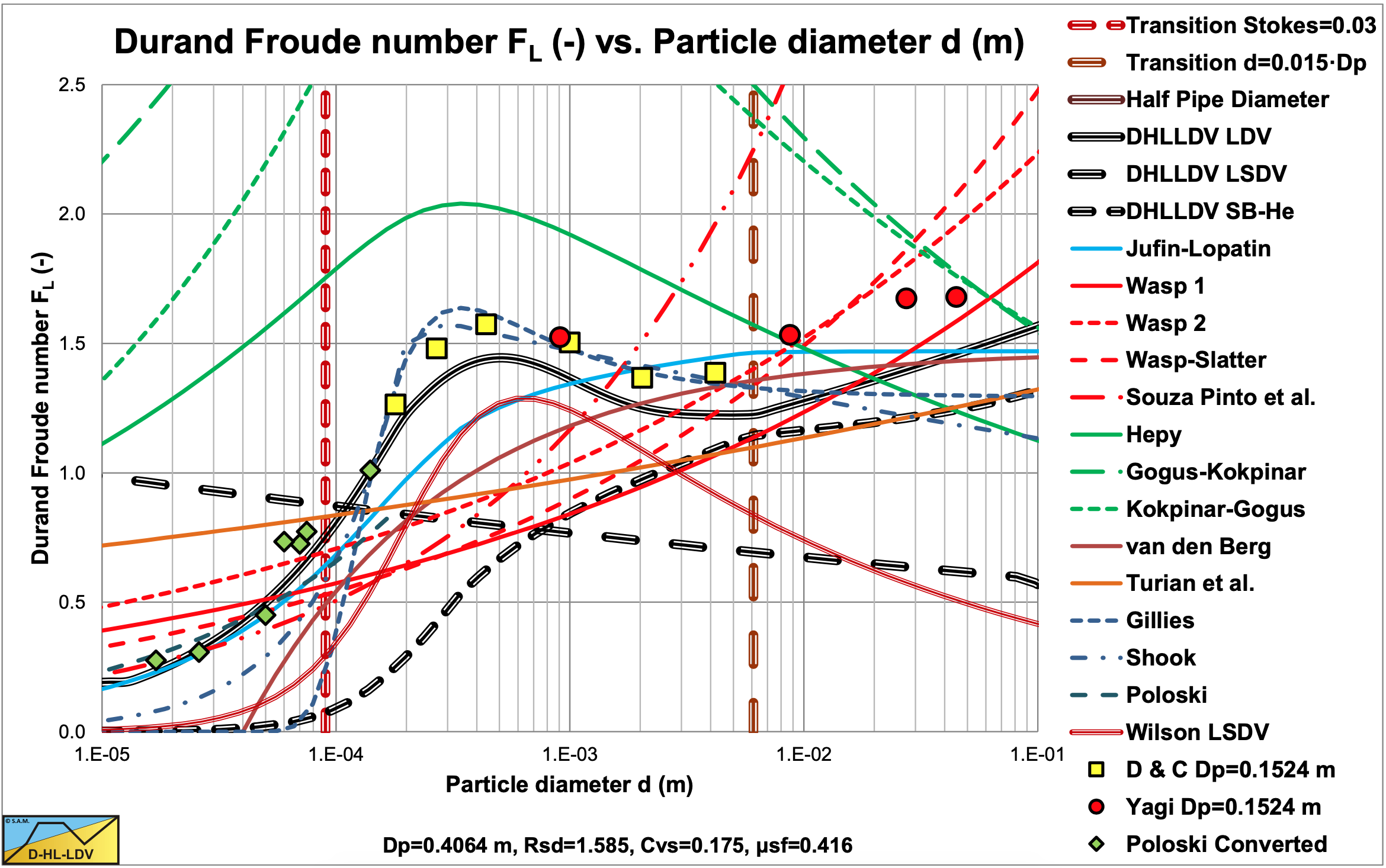
Figure 6.27-2, Figure 6.27-3, Figure 6.27-4 and Figure 6.27-5 show the Limit Deposit Velocities of DHLLDV (see Chapter 7), Durand & Condolios (1952), Jufin & Lopatin (1966), Wasp et al. (1970), Wasp & Slatter (2004), Souza Pinto et al. (2014), Hepy et al. (2008), Gogus & Kokpinar (1993), Kokpinar & Gogus (2001), van den Berg (1998), Turian et al. (1987) and Gillies (1993) for 4 pipe diameters. The curves of Hepy et al. (2008), Gogus & Kokpinar (1993) and Kokpinar & Gogus (2001) show a maximum FL value for particles with a diameter near d=0.5 mm. However these models show an increasing FL value with the pipe diameter, which contradicts the numerous experimental data, showing a slight decrease. The models of Turian et al. (1987) , Wasp et al. (1970), Wasp & Slatter (2004) and Souza Pinto et al. (2014) show an increasing FL value with increasing particle diameter and a slight decrease with the pipe diameter. Jufin & Lopatin (1966) show an increase with the particle diameter and a slight decrease with the pipe diameter (power -1/6). The model of van den Berg (1998) shows an increasing FL with the particle diameter, but no dependency on the pipe diameter. Durand & Condolios (1952) did not give an equation but a graph. The data points as derived from the original publication in (1952) (Low Correct) and from Durand (1953) (High Incorrect) are shown in the graphs. The data points show a maximum for d=0.5 mm. They did not report any dependency on the pipe diameter. The model of Gillies (1993) tries to quantify the Durand & Condolios (1952) data points (but the incorrect ones) but does not show any dependency on the pipe diameter for the FL Froude number. The increase of the FL value with the pipe diameter of the Hepy et al. (2008), Gogus & Kokpinar (1993) and Kokpinar & Gogus (2001) models is probably caused by the forced d/Dp relation. With a strong relation with the particle diameter and a weak relation for the pipe diameter, the pipe diameter will follow the particle diameter. Another reason may be the fact that they used pipe diameters up to 0.1524 m (6 inch) and the smaller the pipe diameter the more probable the occurrence of a sliding bed and other limiting conditions.
The figures show that for small pipe diameters all models are close. The reason is probably that most experiments are carried out with small pipe diameters. Only Jufin & Lopatin (1966) covered a range from 0.02 m to 0.9 m pipe diameters. Recently Thomas (2014) gave an overview and analysis of the LDV (or sometimes the LSDV). He repeated the findings that the LDV depends on the pipe diameter with a power smaller than 0.5 but larger than 0.1. The value of 0.1 is for very small particles, while for normal sand and gravels a power is expected between 1/3 according to Jufin & Lopatin (1966) and 1/2 according to Durand & Condolios (1952). Most equations are one term equations, making it impossible to cover all aspects of the LDV behavior. Only Gillies (1993) managed to construct an equation that gets close. The Gillies (1993) equation would be a good alternative in a modified form, incorporating the pipe diameter and relative submerged density effects, valid for particle with d>0.2 mm, like:
\[\ \mathrm{v}_{\mathrm{l s}, \mathrm{ld v}}=\mathrm{1 .0 5 \cdot \mathrm { e }}^\left({0 . 5 1 - 0 . 0 0 7 3 \cdot \mathrm { C } _ { \mathrm { D } } - \mathrm { 1 2 . 5 } \cdot \left( \frac { ( { \mathrm{g} \cdot v } _ { \mathrm { l } } ) ^ { 2 / 3 } } { \mathrm { g . d } } - \mathrm { 0 . 1 4 } \right) ^ { 2 }}\right) \cdot(\mathrm{2 \cdot g \cdot D _ { \mathrm { p } } \cdot \mathrm { R } _ { \mathrm { s d } } ) ^ { \mathrm { 0 . 4 2 } } \cdot \left( \frac { \mathrm { 1 .5 8 5 } } { \mathrm { R } _ { \mathrm { s d } } } \right) ^ { \mathrm { 0 .1 2 } }}\]
With the Froude number FL:
\[\ \mathrm{F_{L}=\frac{v_{l s, l d v}}{\sqrt{2 \cdot g \cdot D_{p} \cdot R_{s d}}}}=1.05 \cdot \frac{\mathrm{e}^\left({0.51-0.0073 \cdot \mathrm{C_{D}}-12.5 \cdot\left(\frac{\left(\mathrm{g} \cdot v_{\mathrm{l}}\right)^{2 / 3}}{\mathrm{g \cdot d}}-0.14\right)^{2}}\right)}{\left(\mathrm{2 \cdot g \cdot D_{p} \cdot R_{s d}}\right)^{0.08}}{ \cdot\left(\frac{1.585}{\mathrm{R_{s d}}}\right)^{0.12}}\]
Lately Lahiri (2009) performed an analysis using artificial neural network and support vector regression. Azamathulla & Ahmad (2013) performed an analysis using adaptive neuro-fuzzy interference system and gene- expression programming. Although these methodologies may give good correlations, they do not explain the physics. Lahiri (2009) however did give relations for the volumetric concentration, the particle diameter, the pipe diameter and the relative submerged density.
Resuming, the following conclusions can be drawn for sand and gravel:
- The LDV is proportional to the pipe diameter to a power between 1/3 and 1/2 (about 0.4).
- The LDV has a lower limit for very small particles, after which it increases to a maximum at a particle diameter of about d=0.5 mm.
- For larger particles the LDV decreases to a particle diameter of about 2 mm.
- For very large particles the LDV remains constant.
- For particles d>0.015·Dp, the LDV increases again. This limit is however questionable and requires more research.
The relation between the LDV and the relative submerged density is not very clear, however the data shown by Kokpinar & Gogus (2001) and the conclusions of Lahiri (2009) show that the FL value decreases with increasing solids density and thus relative submerged density Rsd to a power of -0.2 to -0.4.
The volumetric concentration leading to the maximum LDV is somewhere between 15% and 25%, depending on the particle diameter. For small concentrations a minimum LDV is observed by Durand & Condolios (1952). This minimum LDV increases with the particle diameter and reaches the LDV of 20% at a particle diameter of 2 mm with a pipe diameter of 0.1524 m (6 inch).
For the dredging industry the Jufin & Lopatin (1966) equation gives a good approximation for sand and gravel, although a bit conservative. The model of van den Berg (1998) is suitable for large diameter pipes as used in dredging sand and/or gravel, but underestimates the LDV for pipe diameters below 0.8 m. Both models tend to underestimate the LDV for particle diameters below 1 mm.
Analyzing the literature, equations and experimental data, the LDV can be divided into a number of regimes for sand and gravel:
- Very small particles, smaller than about 50% of the thickness of the viscous sub layer, a lower limit of the LDV. This is for particles up to about 0.015 mm in large pipes to 0.04 mm in very small pipes.
- Small particles up to about 0.15 mm, a smooth bed, show an increasing LDV with increasing particle diameter.
- Medium particles with a diameter from 0.15 mm up to a diameter of 2 mm, a transition zone from a smooth bed to a rough bed. First the LDV increases to a particle diameter of about 0.5 mm, after which it decreases slowly to an asymptotic value at a diameter of 2mm.
- Large particles with a diameter larger than 2 mm, a rough bed, giving a constant LDV.
- Particles with a particle diameter to pipe diameter ratio larger than about 0.015 cannot be carried by turbulent eddies, just because the eddies are not large enough. This will probably result in an increasing LDV with the particle diameter.
The above conclusions are the starting points of the DHLLDV Limit Deposit Velocity Model as derived and described in Chapter 7 and already shown in the figures.
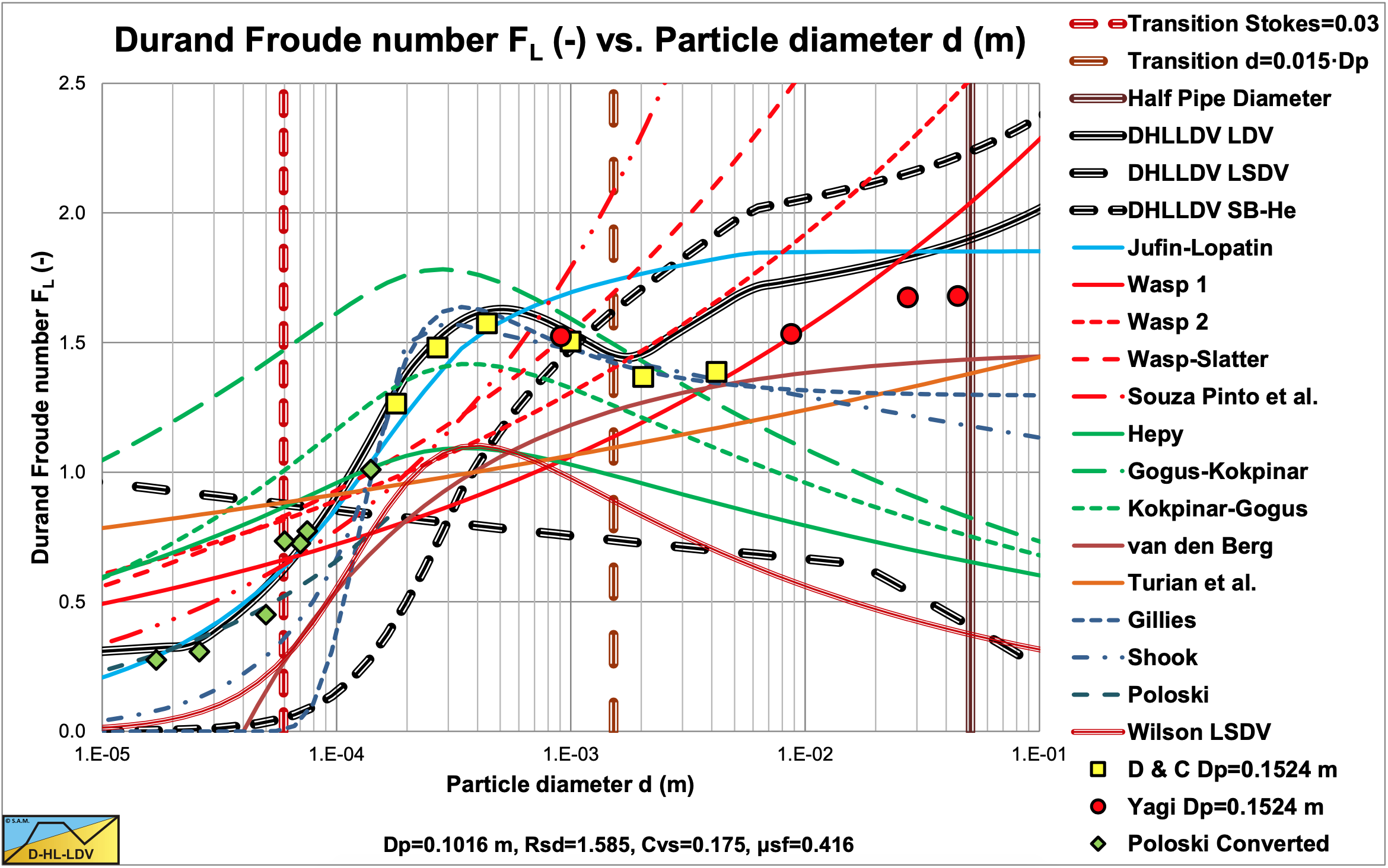
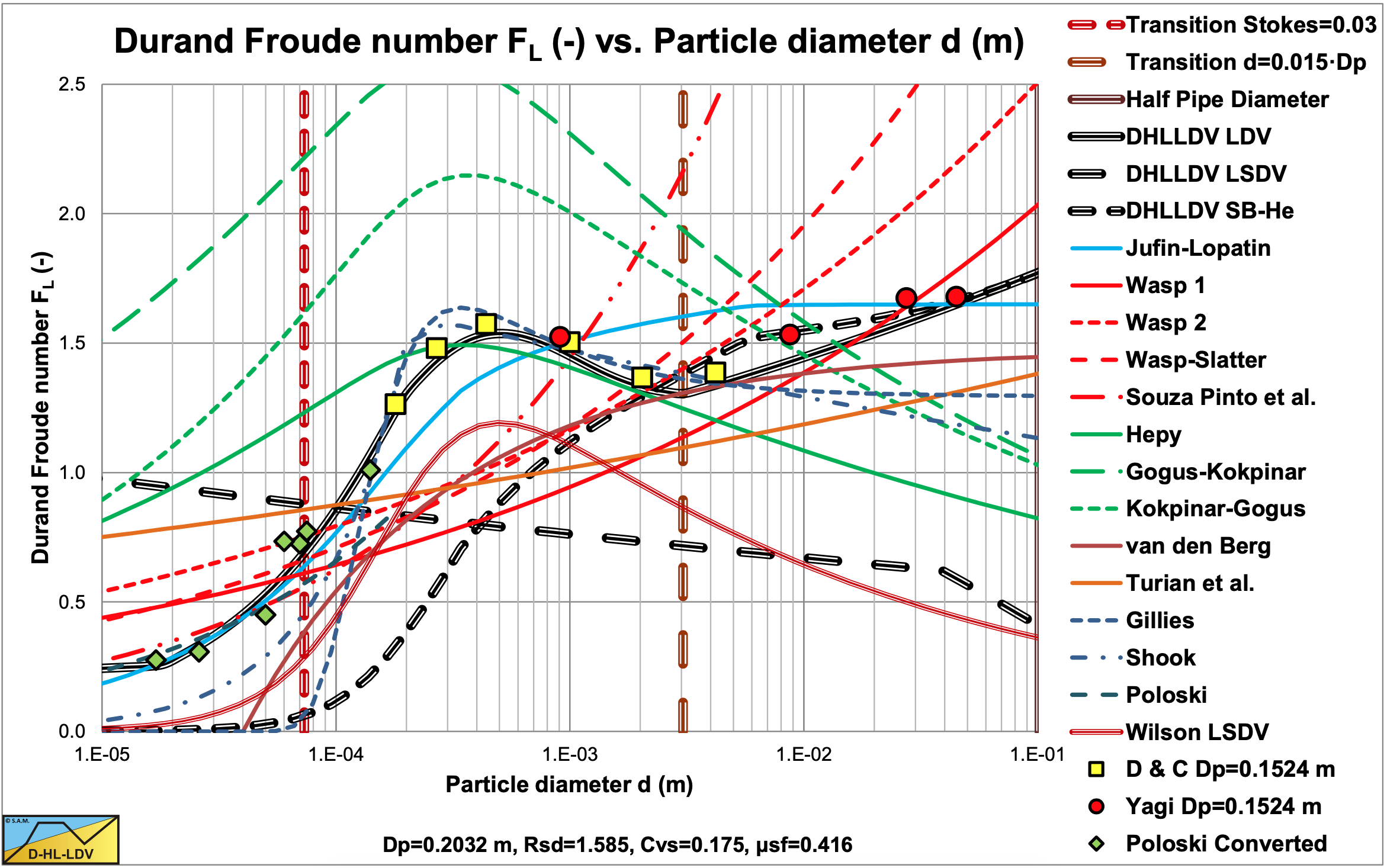
The LSDV curve in these figures shows the start of a sliding bed. The Sb-He curve shows the transition of a sliding bed to heterogeneous flow. The intersection point of these two curves shows the start of occurrence of a sliding bed. For smaller particles a sliding bed will never occur, because the particles are already suspended before the bed can start sliding. Larger particles will show a sliding bed. It is also clear that the Wilson LSDV curve is considerably lower than the DHLLDV curve, the Durand & Condolios, Yagi et al. and Poloski data for the smaller pipe diameters. It should be mentioned that the Wilson LSDV curve is the maximum curve at a concentration of about 10%. Other concentrations will show lower curves. The DHLLDV curve is also the maximum curve.
6.27.30 Nomenclature Limit Deposit Velocity
|
Ar |
Archimedes number |
- |
|
CD |
Particle drag coefficient |
- |
|
Cvs |
Spatial volumetric concentration |
- |
|
Cvt |
Delivered (transport) volumetric concentration |
- |
|
d |
Particle diameter |
m |
|
d50 |
Particle diameter 50% passing |
m |
|
Dp |
Pipe diameter |
m |
|
Erhg |
Relative excess hydraulic gradient |
- |
|
FL |
Durand & Condolios LDV Froude number |
- |
|
Fdown |
Downwards force on particle, gravity |
kN |
|
Fup |
Upwards force on particle, drag |
kN |
|
g |
Gravitational constant (9.81 m/s2) |
m/s2 |
|
im |
Mixture hydraulic gradient |
m/m |
|
il |
Liquid hydraulic gradient |
m/m |
|
ΔL |
Length of pipe segment considered |
m |
|
LDV |
Limit Deposit Velocity |
m/s |
|
LSDV |
Limit of Stationary Deposit Velocity |
m/s |
|
MHGV |
Minimum Hydraulic Gradient V elocity |
m/s |
|
n |
Power hindered settling |
- |
|
N |
Zandi & Govatos parameter |
- |
|
P |
Power dissipated per unit mass of liquid |
kW |
|
Rsd |
Relative submerged density (sand 1.65) |
- |
|
u* |
Friction velocity |
m/s |
|
vef |
Eddy fluctuation velocity |
m/s |
|
vls |
Line speed |
m/s |
|
vls,ldv |
Limit Deposit Velocity |
m/s |
|
vSB-He |
Transition sliding bed regime with heterogeneous regime |
m/s |
|
vt |
Terminal settling velocity |
m/s |
|
α |
Correction factor eddy velocity |
- |
|
β |
Hindered settling power, Richardson & Zaki |
- |
|
ρl |
Density liquid |
ton/m3 |
|
ρs |
Density solids |
ton/m3 |
|
ρm |
Density mixture |
ton/m3 |
|
ψ |
Shape factor |
- |
|
ψ* |
Jufin Lopatin particle Froude number |
- |
|
μsf |
Sliding friction coefficient |
- |
| \(\ v_{\mathrm{l}}\) |
Kinematic viscosity liquid |
m2/s |
|
λl |
Darcy Weisbach friction factor |
- |
|
θ |
Pipe inclination angle |
rad |