6.29: Starting Points DHLLDV Framework

The DHLLDV Framework, as will be described in the next chapter, has starting points based on analysis of all models investigated in this chapter and based on the fundamentals. Most starting points are based on experiments and models for sand and gravel, although also other solids are investigated.

6.29.1 The Liquid Properties

If the solids contain fines, the liquid properties have to be adjusted. The dynamic viscosity and the liquid density are influence by this. A number of models deal with graded solids with a high fraction of fines. So for these models the adjustment is essential. The definition of fines is not very clear. Often a particle diameter is used, however it also seems to make sense to use a particle diameter to pipe diameter ratio, since the size of eddies also depends on the pipe diameter. In true homogeneous flow both the liquid viscosity and the liquid density have to be adjusted. In pseudo homogeneous flow only the liquid density. Usually the equations of D.G. Thomas (1965) are used for this. The liquid property adjustments have to be carried out before identifying flow regimes.

6.29.2 Possible Flow Regimes

There are 5 main flow regimes identified, most also identified by other researchers. These are:

1. The stationary bed flow regime, with or without sheet flow or suspension.
2. The sliding bed flow regime, usually with sheet flow or suspension.
3. The heterogeneous flow regime.
4. The homogeneous flow regime.
5. The sliding flow regime or stratified flow regime.

Figure 6.29-1: Flow regimes according to Durand & Condolios (1952) and Newitt et al. (1955), modified. (Captions for the 36 inch pipe diameter, C_v=0.15).

When starting at line speed zero and increasing the line speed, not all flow regimes have to occur, depending on the particle size and the particle size to pipe diameter ratio. It also matters whether a constant spatial volumetric concentration or a constant delivered volumetric concentration is considered.

For a constant spatial volumetric concentration, the following scenarios are possible.

1. Fine particles and a small d/D_p ratio. A stationary bed without sheet flow or suspension, a stationary bed with sheet flow or suspension, heterogeneous flow and (pseudo) homogeneous flow.
2. Medium/coarse particles and a small/medium d/D_p ratio. A stationary bed without sheet flow or suspension, a stationary bed with sheet flow or suspension, a sliding bed with sheet flow or suspension, heterogeneous flow and (pseudo) homogeneous flow.
3. Very coarse particles and a large d/D_p ratio. A stationary bed without sheet flow or suspension, a stationary bed with sheet flow or suspension, a sliding bed with sheet flow or suspension, sliding/stratified flow and (pseudo) homogeneous flow.

For a constant delivered volumetric concentration, the following scenarios are possible.

1. Fine particles and a small d/D_p ratio. A stationary bed with sheet flow or suspension, a sliding bed with sheet flow or suspension, heterogeneous flow and (pseudo) homogeneous flow.
2. Medium/coarse particles and a small/medium d/D_p ratio. A stationary bed with sheet flow or suspension, a sliding bed with sheet flow or suspension, heterogeneous flow and (pseudo) homogeneous flow.
3. Very coarse particles and a large d/D_p ratio. A stationary bed with sheet flow or suspension, a sliding bed with sheet flow or suspension, sliding/stratified flow and (pseudo) homogeneous flow.

6.29.3 Flow Regime Behavior

For a constant spatial volumetric concentration, the following flow regime behavior is observed:

1. In the stationary bed regime the hydraulic gradient increases with the square of the line speed until sheet flow starts to occur, after which it increases with the line speed to a higher power.
2. In the sliding bed regime the excess hydraulic gradient does not depend on the line speed. It does however depend on the sliding friction factor and the relative submerged density and of course on the spatial concentration. The dependency on the spatial concentration as described by Wilson et al. (2006), the hydrostatic normal stress approach, has not been observed. Instead a linear dependency with the volumetric concentration is observed. The excess hydraulic gradient does not depend on the particle size, but there could be some relation between the particle size and the sliding friction factor. There could also be a relation between the particle size to pipe diameter ratio and the sliding friction factor.
3. In the heterogeneous regime the excess hydraulic gradient is reversely proportional to the line speed with a power varying from -1 to -2. Most researchers found a value close to -1, but some researchers use more negative powers up to -1.86 (Zandi & Govatos (1967)). One can say in general, the more uniform the solids, the more negative the power.
4. In the homogeneous regime everybody agrees that the excess hydraulic gradient is between zero and the ELM excess hydraulic gradient. There are different formulations to quantify this, but no general rule could be found. It does seem however that the higher the concentration, the lower the excess hydraulic gradient, using a scale of 0 to 1 from the pure liquid excess hydraulic gradient (0) to the ELM excess hydraulic gradient (1). The new methodology of Talmon (2011), assuming a particle free viscous sub-layer, seems promising to quantify this effect.
5. The sliding flow regime or fully stratified regime has not been identified as such, but has been observed by many researchers. This flow regime occurs when the concentration of the bed becomes so small that one cannot speak of a bed anymore, but the particles are still stratified and the excess hydraulic gradient behaves like a sliding bed. It has been observed that this occurs above a certain particle diameter to pipe diameter ratio and above some threshold concentration (5%-6%). Wilson et al. (2006) suggests using a power of -0.25 for the relation between the excess hydraulic gradient and the line speed.

For a constant delivered volumetric concentration, the following behavior is observed:

1. At very low line speeds a combination of a stationary bed with a moving bed above and suspension above the moving bed is observed. A 3 layer or multi-layer model is required. The spatial volumetric concentration will increase with decreasing line speed to the bed concentration, resulting in a maximum excess hydraulic gradient based on a pipe filled 100% with bed. This is not in a range of normal operational parameters, so most researchers did not carry out experiments in this range and did not discover this asymptotic behavior.
2. At a still low line speed the whole bed starts moving and a 2 layer model gives a good prediction. The excess hydraulic gradient decreases with the line speed to a small negative power, less negative than -1. The higher the line speed, the higher the bed velocity and the larger the fraction of particles in suspension or in a sheet flow layer.
3. Above a certain line speed the sliding bed behavior has a transition to heterogeneous behavior, where the excess hydraulic gradient is reversely proportional to the line speed with a power slightly more negative than in the constant spatial volumetric concentration situation. Since most experiments are carried out with delivered volumetric concentration measurements, it is not always clear whether the powers observed (-1 to - 2) are for delivered or spatial volumetric concentrations.
4. At higher line speeds in the homogeneous or pseudo homogeneous regimes, the spatial and delivered concentrations are almost equal and the same behavior is observed.
5. At higher line speeds in the sliding flow regime, the spatial and delivered concentrations are almost equal and the same behavior is observed.

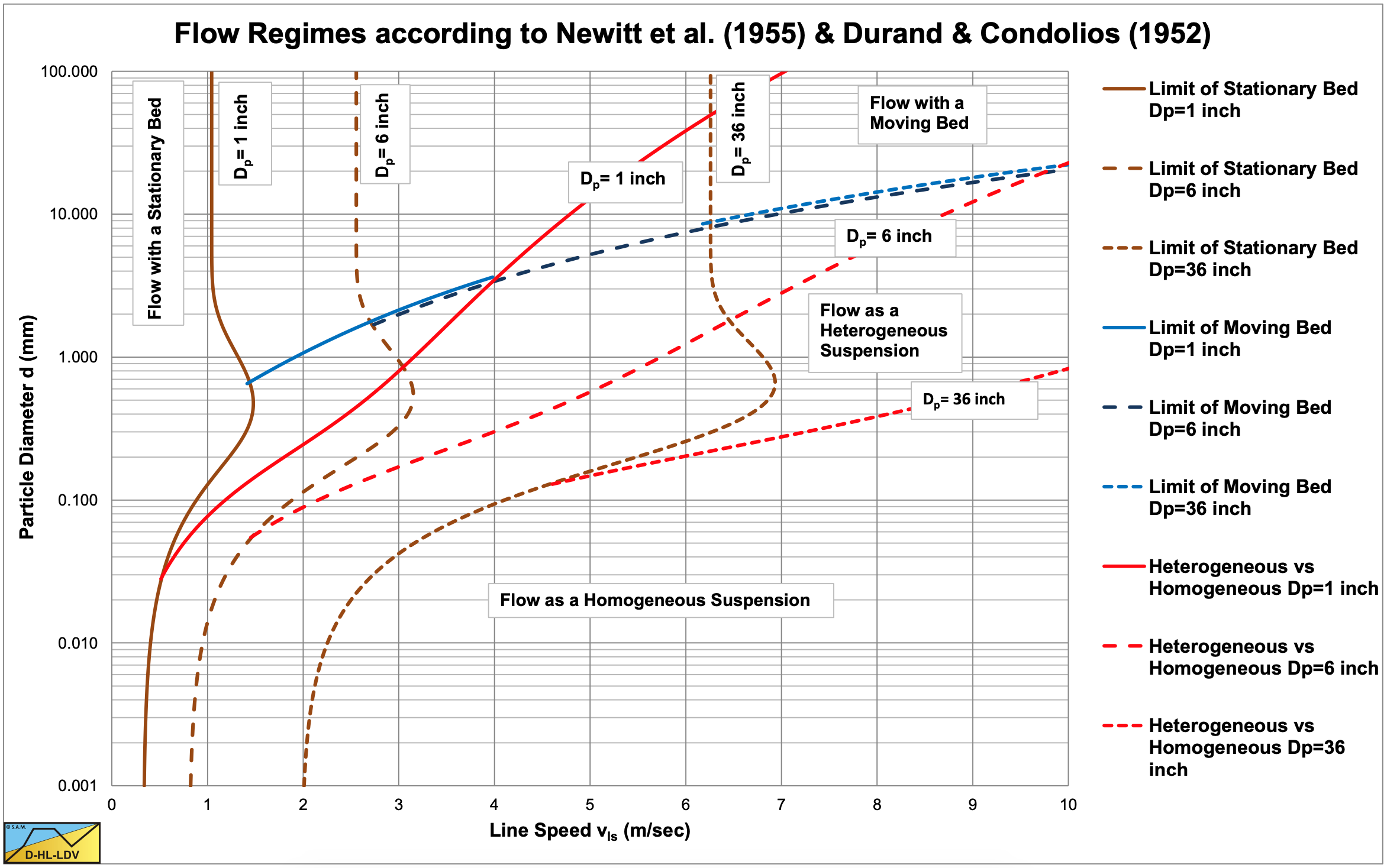
6.29.4 The LSDV, LDV and MHGV

Many definitions exist for the line speed above which there is no bed. The Limit of Stationary Deposit Velocity (LSDV) is the velocity above which the bed is sliding and below which the bed is stationary. The Limit Deposit Velocity (LDV) is the velocity above which there is no stationary or sliding bed. The Minimum Hydraulic Gradient Velocity (MHGV) is the line speed where the hydraulic gradient is at a minimum. It is observed that fine particles often do not result in a sliding bed but have a direct transition from a stationary bed to heterogeneous transport. The bed vaporizes by particle suspension. Coarser particle will have a transition from a stationary bed (with sheet flow) to a sliding bed (LSDV) to heterogeneous transport. The occurrence of a sliding bed also depends on the particle diameter to pipe diameter ratio. In very small diameter pipes (1 inch) almost every normal particle diameter in sand will result in a sliding bed. However in large diameter pipes (1 m) as used in dredging, particles have to be very coarse (gravel) to result in a sliding bed. So in this case most sand particles will have a direct transition from a stationary bed to heterogeneous transport. The LSDV does not exist in the latter case, the LDV always exists. In general the LDV depends on the particle diameter, the pipe diameter and the volumetric concentration. Different researchers found that the maximum LDV occurs at a volumetric concentration between 10% and 20%, probably closer to 20%. They also found that the LDV increases with the pipe diameter to a power between 1/3 and 1/2.

The relation with the particle diameter is more complex.
For very fine particles, fitting in the viscous sub-layer, a lower limit to the LDV is found. This lower limit does not depend on the particle diameter and only weak (power 0.1) on the pipe diameter, since the thickness of the viscous sub-layer depends weak on the pipe diameter.
For fine particles the LDV increases with the particle diameter up to a particle diameter of about 0.5 mm where a maximum is reached.
Medium to coarse particles first show a decrease of the LDV with increasing particle diameter, after which the LDV remains constant.
For a large particle diameter to pipe diameter ratio (>0.015) it looks like the LDV is increasing again with the particle diameter. It is the question however what is the value of the LDV here, since in this case the sliding flow regime will occur and the value of the LDV is more the MHGV, just a number to use in calculations without a real physical meaning.
There also seems to be a lower limit to the LDV over the whole range of particle diameters. It looks like this lower limit is caused by the transition between the sliding bed regime and the heterogeneous regime. This lower limit has hardly any effect on the LDV of fine particles, since the sliding bed regime will not occur there, but it will have a strong effect on medium and coarse particles in small diameter pipes, where the sliding bed regime is most likely to occur.

6.29.5 The Slip Velocity or Slip Ratio

The slip velocity has two definitions. First the slip velocity is the difference between the solids velocity and the liquid velocity. Second the slip velocity is the difference between the solids velocity and the line speed, the cross sectional averaged mixture velocity. For small concentrations there is not much difference, but for large concentrations there is. Since the line speed is one of the inputs of every model, the second definition is used, but one should consider this is not 100% correct scientifically.

The slip ratio is defined here as the ratio of the slip velocity to the line speed. So a slip ratio of 1 means the particles have no velocity, while a slip ratio of 0 means the particles move with the line speed.
Above the LDV the slip ratio is relatively small, depending on the particle properties. In the homogeneous regime the slip ratio will be close to zero. Below the LDV the slip ratio will increase with decreasing line speed. Not to 1 as many understand, but to a value depending on the delivered concentration.

Suppose the delivered concentration equals the bed concentration at line speeds close to zero, so the whole pipe is filled with a bed, this means the bed will have a velocity equal to the line speed and the slip ratio equals zero.

Now suppose the delivered concentration is almost zero, so almost pure liquid being transported. At line speeds close to zero there will be a stationary of slowly sliding bed, but the bed velocity must be almost zero, otherwise the delivered concentration cannot be close to zero. So a pipe almost fully occupied with bed and hardly any delivered concentration, results in a slip ratio of almost 1. The asymptotic value of the slip ratio for a delivered concentration approaching zero is equal to 1.

Now suppose the delivered concentration is 50% of the bed concentration. At line speeds close to zero there will be a stationary of slowly sliding bed with some space above it transporting the mixture. The spatial concentration in the pipe is almost the bed concentration, since the pipe is almost completely occupied with bed, but the delivered concentration is 50% of the bed concentration. This means that on average the particles move with 50% of the line speed, giving a slip ratio of 0.5.

This means that the maximum slip ratio equals (1-C_vt/C_vb) at line speed zero, decreasing to a certain value at the LDV. Above the LDV the slip ratio will decrease rapidly. From the observations the conclusion can be drawn that the slip ratio decreases slowly in the sliding bed regime, but rapidly the closer the line speed gets to the LDV.

6.29.6 The Concentration Distribution

The concentration distribution in a pipe gives information about the internal structure of the flow. Not many researchers report experimental concentration distributions, but some do. In general the concentration distribution is not part of the head loss models or equations, but in the Wasp or Wasp related models it is. The measured concentration distributions are usually predicted with solutions of the advection diffusion equations for open channel flow. Often these equations can be solved analytically, resulting in convenient equations. For pipe flow however the equations have to be solved numerically and also integrated numerically in order to find the correct cross section averaged spatial concentration.

The concentration distribution depends on the terminal settling velocity and the diffusivity. Often the non-hindered terminal settling velocity and some known diffusivity or diffusivity distribution are used. This however does not give satisfying results. Using the hindered settling velocity and a particle diameter and concentration dependent diffusivity gives better results. Kaushal & Tomita (2002B) found relations for this. Using the local hindered terminal settling velocity and concentration gives even better results.

6.29.7 The Dimensionless Numbers used

The use of dimensionless numbers in the head loss models, especially the models for the heterogeneous regime, and in the LDV models is dangerous and misleading. In a number of models the flow Froude number and the particle Froude number are used. Also the particle diameter to pipe diameter ratio is often used. In these numbers the ratio between different independent parameters is present. For example the velocity divided by the square root of a diameter in the Froude number. When one of these parameters is varied over a wide range, while the other parameter is only varied over a small range, using the dimensionless number may give a good correlation in a regression. However when the parameter with the small range is used outside that range, unexpected results may appear. This is observed with the flow Froude number resulting in a proportionality of the head losses with the pipe diameter which is not correct, but also with the Durand Froude number for the LDV and the particle diameter to pipe diameter ratio, resulting in a relation of the LDV with the pipe diameter which is not correct. It is better to start unbiased with all independent parameters based on physics. If the result is dimensionless numbers in the equations, it may be convenient.

6.29.8 The Type of Graph used

Usually head loss graphs are shown with the line speed on the abscissa and the hydraulic gradient on the ordinate. This is convenient in combination with pump head curves to determine the working point, by multiplying the hydraulic gradient with ρ_l·g·ΔL. However if experiments are carried out with different concentrations also giving some scatter, a messy graph is the result. The graph is not non-dimensional and it is difficult to compare different experiments. Using another type of graph mainly solves this problem. Using the relative excess hydraulic gradient on the ordinate and the liquid hydraulic gradient on the abscissa on double logarithmic coordinates, creates an almost dimensionless graph. Almost, because some flow regimes are still more or less concentration dependent. Another advantage is that lines that are (power) curved in the hydraulic gradient versus line speed graph, become straight lines in the double logarithmic relative excess hydraulic gradient versus liquid hydraulic gradient graph. For the LDV a graph is used with the Durand Froude number F_L on the linear ordinate and the particle diameter on the logarithmic abscissa. In this graph the F_L value only depends slightly on the pipe diameter, with a power of about -0.1.