6.8: Analytical and Numerical Water Pore Pressure Calculations

As is shown in Figure 6-9, the water can flow from 4 directions to the shear zone where the dilatancy takes place. Two of those directions go through the sand which has not yet been deformed and thus have a permeability of ki, while the other two directions go through the deformed sand and thus have a permeability of k_max. Figure 6-12 shows that the flow lines in 3 of the 4 directions have a more or less circular shape, while the flow lines coming from above the blade have the character of a straight line. If a point on the shear zone is considered, then the water will flow to that point along the 4 flow lines as mentioned above. Along each flow line, the water will encounter a certain resistance. One can reason that this resistance is proportional to the length of the flow line and reversibly proportional to the permeability of the sand. Figure 6-20 shows a point on the shear zone and it shows the 4 flow lines. The length of the flow lines can be determined with the equations (6-36), (6-37), (6-38) and (6-39). The variable L_max in these equations is the length of the shear zone, which is equal to h_i/sin(β), while the variable L starts at the free surface with a value zero and ends at the blade tip with a value L_max.

According to the law of Darcy, the specific flow q is related to the pressure difference Δp according to:

\[\ \mathrm{q}=\mathrm{k} \cdot \mathrm{i}=\mathrm{k} \cdot \frac{\Delta \mathrm{p}}{\rho_{\mathrm{w}} \cdot \mathrm{g} \cdot \Delta \mathrm{s}}\tag{6-34}\]

The total specific flow coming through the 4 flow lines equals the total flow caused by the dilatation, so:

\[\ \begin{array}{left}\mathrm{q}=\varepsilon \cdot \mathrm{v}_{\mathrm{c}} \cdot \sin (\beta)\\
=\mathrm{k}_{\max } \cdot \frac{\Delta \mathrm{p}}{\rho_{\mathrm{w}} \cdot \mathrm{g} \cdot \mathrm{s}_{1}}+\mathrm{k}_{\mathrm{m a x}} \cdot \frac{\Delta \mathrm{p}}{\rho_{\mathrm{w}} \cdot \mathrm{g} \cdot \mathrm{s}_{2}}+\mathrm{k}_{\mathrm{i}} \cdot \frac{\Delta \mathrm{p}}{\rho_{\mathrm{w}} \cdot \mathrm{g} \cdot \mathrm{s}_{3}}+\mathrm{k}_{\mathrm{i}} \cdot \frac{\Delta \mathrm{p}}{\rho_{\mathrm{w}} \cdot \mathrm{g} \cdot \mathrm{s}_{4}}\end{array}\tag{6-35}\]

Figure 6-20: The flow lines used in the analytical method.

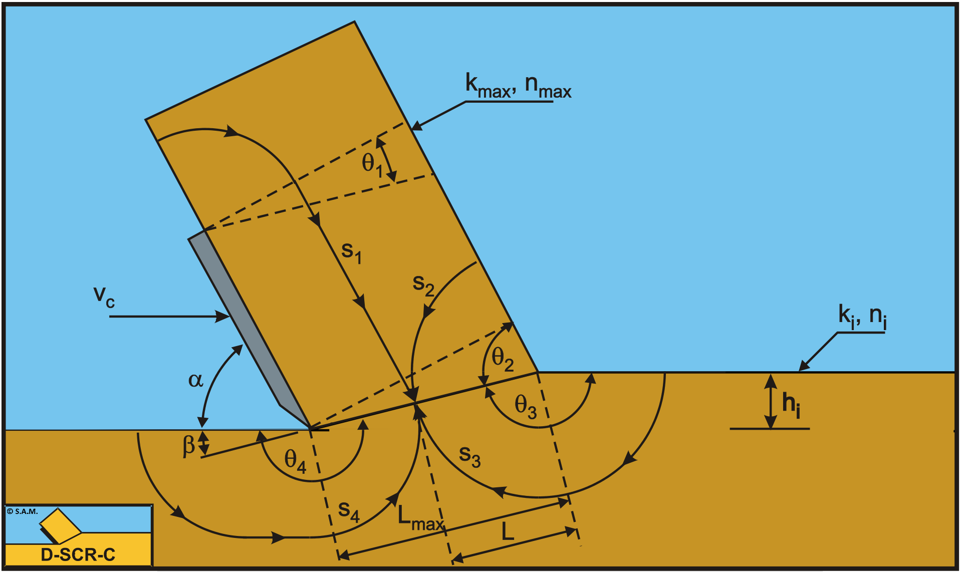
For the lengths of the 4 flow lines, where s₂ and s₃ have a correction factor of 0.8 based on calibration with the experiments:

\[\ \begin{array}{left} \mathrm{s}_{1}=\left(\mathrm{L}_{\mathrm{m} \mathrm{a} \mathrm{x}}-\mathrm{L}\right) \cdot\left(\frac{\pi}{2}+\theta_{1}\right)+\frac{\mathrm{h}_{\mathrm{b}}}{\sin (\alpha)}\\
\text{With : }\quad \theta_{1}=\frac{\pi}{2}-(\alpha+\beta)\end{array}\tag{6-36}\]

\[\ \begin{array}{left} \mathrm{s}_{2}=\mathrm{0.8} \cdot \mathrm{L} \cdot \mathrm{\theta}_{2}\\
\text{With : }\quad \theta_{2}=\alpha+\beta\end{array}\tag{6-37}\]

\[\ \begin{array}{left} \mathrm{s}_{\mathrm{3}}=\mathrm{0 .8 \cdot L \cdot \theta _ { 3 }}\\
\text{With : }\quad \theta_{3}=\pi-\beta\end{array}\tag{6-38}\]

\[\ \begin{array}{left}\mathrm{s}_{4}=\left(\mathrm{L}_{\mathrm{m a x}}-\mathrm{L}\right) \cdot \theta_{4}+\mathrm{0 .9} \cdot \mathrm{h}_{\mathrm{i}} \cdot\left(\frac{\mathrm{h}_{\mathrm{i}}}{\mathrm{h}_{\mathrm{b}}}\right)^{0.5} \cdot(\mathrm{1 .8 5} \cdot \mathrm{\alpha})^{2} \cdot\left(\frac{\mathrm{k}_{\mathrm{i}}}{\mathrm{k}_{\mathrm{m a x}}}\right)^{0.4}\\
\mathrm{W i t h}: \quad \theta_{4}=\pi+\beta\end{array}\tag{6-39}\]

The equation for the length s₄ has been determined by calibrating this equation with the experiments and with the FEM calculations. This length should not be interpreted as a length, but as the influence of the flow of water around the tip of the blade. The total specific flow can also be written as:

\[\ \begin{array}{left}\rho_{\mathrm{w}} \cdot \mathrm{g} \cdot \mathrm{q}=\rho_{\mathrm{w}} \cdot \mathrm{g} \cdot \mathrm{\varepsilon} \cdot \mathrm{v}_{\mathrm{c}} \cdot \sin (\beta)\\
=\frac{\Delta \mathrm{p}}{\left(\frac{\mathrm{s}_{1}}{\mathrm{k}_{\max }}\right)}+\frac{\Delta \mathrm{p}}{\left(\frac{\mathrm{s}_{2}}{\mathrm{k}_{\max }}\right)}+\frac{\Delta \mathrm{p}}{\left(\frac{\mathrm{s}_{3}}{\mathrm{k}_{\mathrm{i}}}\right)}+\frac{\Delta \mathrm{p}}{\left(\frac{\mathrm{s}_{4}}{\mathrm{k}_{\mathrm{i}}}\right)}=\frac{\Delta \mathrm{p}}{\mathrm{R}_{1}}+\frac{\Delta \mathrm{p}}{\mathrm{R}_{2}}+\frac{\Delta \mathrm{p}}{\mathrm{R}_{3}}+\frac{\Delta \mathrm{p}}{\mathrm{R}_{4}}=\frac{\Delta \mathrm{p}}{\mathrm{R}_{\mathrm{t}}}\end{array}\tag{6-40}\]

The total resistance on the flow lines can be determined by dividing the length of a flow line by the permeability of the flow line. The equations (6-41), (6-42), (6-43) and (6-44) give the resistance of each flow line.

\[\ \mathrm{R}_{1}=\frac{\mathrm{s}_{1}}{\mathrm{k}_{\mathrm{m} \mathrm{a x}}}\tag{6-41}\]

\[\ \mathrm{R}_{2}=\frac{\mathrm{s}_{2}}{\mathrm{k}_{\mathrm{m a x}}}\tag{6-42}\]

\[\ \mathrm{R}_{3}=\frac{\mathrm{s}_{\mathrm{3}}}{\mathrm{k}_{\mathrm{i}}}\tag{6-43}\]

\[\ \mathrm{R}_{4}=\frac{\mathrm{s}_{4}}{\mathrm{k}_{\mathrm{i}}}\tag{6-44}\]

Since the 4 flow lines can be considered as 4 parallel resistors, the total resulting resistance can be determined according to the rule for parallel resistors. Equation (6-45) shows this rule.

\[\ \frac{1}{\mathrm{R}_{\mathrm{t}}}=\frac{\mathrm{1}}{\mathrm{R}_{\mathrm{1}}}+\frac{\mathrm{1}}{\mathrm{R}_{\mathrm{2}}}+\frac{\mathrm{1}}{\mathrm{R}_{\mathrm{3}}}+\frac{\mathrm{1}}{\mathrm{R}_{\mathrm{4}}}\tag{6-45}\]

The resistance R_t in fact replaces the h_i/k_max part of the equations (6-23), (6-24), (6-28) and (6-29), resulting in equation (6-46) for the determination of the pore vacuum pressure of the point on the shear zone.

\[\ \Delta \mathrm{p}=\rho_{\mathrm{w}} \cdot \mathrm{g} \cdot \mathrm{v}_{\mathrm{c}} \cdot \varepsilon \cdot \sin (\beta) \cdot \mathrm{R}_{\mathrm{t}}\tag{6-46}\]

The average pore vacuum pressure on the shear zone can be determined by summation or integration of the pore vacuum pressure of each point on the shear zone. Equation (6-47) gives the average pore vacuum pressure by summation.

\[\ \mathrm{p}_{1 \mathrm{m}}=\frac{\mathrm{1}}{\mathrm{n}} \cdot \sum_{\mathrm{i}=\mathrm{0}}^{\mathrm{n}} \Delta \mathrm{p}_{\mathrm{i}}\tag{6-47}\]

The determination of the pore pressures on the blade requires a different approach, since there is no dilatation on the blade. However, from the determination of the pore pressures on the shear plane, the pore pressure at the tip of the blade is known. This pore pressure can also be determined directly from:

For the lengths of the 4 flow lines the following is valid at the tip of the blade:

\[\ \mathrm{s_{1}=\frac{h_{b}}{\sin (\alpha)}}\tag{6-48}\]

\[\ \mathrm{s_{2}=0.8 \cdot L_{\max } \cdot \theta_{2} \quad\text{ with : } \quad \theta_{2}=\alpha+\beta}\tag{6-49}\]

\[\ \mathrm{s_{3}=0.8 \cdot L_{\max } \cdot \theta_{3} \quad\text{ with : }\quad \theta_{3}=\pi-\beta}\tag{6-50}\]

\[\ \mathrm{s_{4}=0.9 \cdot h_{\mathrm{i}} \cdot\left(\frac{h_{\mathrm{i}}}{h_{\mathrm{b}}}\right)^{0.5} \cdot(1.85 \cdot \alpha)^{2} \cdot\left(\frac{\mathrm{k}_{\mathrm{i}}}{\mathrm{k}_{\mathrm{max}}}\right)^{0.4}}\tag{6-51}\]

The resistances can be determined with equations (6-41), (6-42), (6-43) and (6-44) and the pore pressure with equation (6-46). Now a linear distribution of the pore pressure on the blade could be assumed, resulting in an average pressure of half the pore pressure at the tip of the blade, but it is not that simple. If the surface of the blade is considered to be a flow line, water will flow from the top of the blade to the tip of the blade. However there will also be some entrainment from the pore water in the sand above the blade, due to the pressure gradient, although the pressure gradient on the blade is considered zero (an impermeable wall). This entrainment flow of water will depend on the ratio of the length of the shear plane to the length of the blade in some way. A high entrainment will result in smaller pore vacuum pressures. When the blade is divided into N intervals, the entrainment per interval will be 1/N times the total entrainment. The two required resistances are now, using i as the counter:

\[\ \mathrm{R}_{1, \mathrm{i}}=\frac{\mathrm{s}_{1, \mathrm{i}}}{\mathrm{k}_{\mathrm{m a x}}} \cdot\left(1-\frac{\mathrm{i}}{\mathrm{N}}\right)\tag{6-52}\]

\[\ \mathrm{R}_{2}=\frac{\mathrm{s}_{2}}{\mathrm{k}_{\mathrm{m a x}}}\tag{6-53}\]

The number of intervals for entrainment and the geometry are taken into account in the constant assumed resistance R₂ according to:

\[\ \mathrm{R}_{2}^{\prime}=\mathrm{N} \cdot \mathrm{1 .7 5} \cdot\left(\frac{\mathrm{h}_{\mathrm{i}}}{\sin (\beta)} \cdot \frac{\sin (\alpha)}{\mathrm{h}_{\mathrm{b}}}\right) \cdot \mathrm{R}_{2}\tag{6-54}\]

The total resistance is now:

\[\ \frac{1}{\mathrm{R}_{\mathrm{t}, \mathrm{i}}}=\frac{\mathrm{1}}{\mathrm{R}_{\mathrm{1}, \mathrm{i}}}+\frac{\mathrm{1}}{\mathrm{R}_{\mathrm{2}}^{\prime}}\tag{6-55}\]

Now starting from the tip of the blade, the initial flows over the blade are determined.

\[\ \mathrm{q}_{0}=\frac{\Delta \mathrm{p}_{\mathrm{tip}}}{\rho_{\mathrm{w}} \cdot \mathrm{g} \cdot \mathrm{R}_{\mathrm{t}, 0}}, \quad \mathrm{q}_{1,0}=\frac{\Delta \mathrm{p}_{\mathrm{tip}}}{\rho_{\mathrm{w}} \cdot \mathrm{g} \cdot \mathrm{R}_{1,0}}, \quad \mathrm{q}_{2,0}=\frac{\Delta \mathrm{p}_{\mathrm{tip}}}{\rho_{\mathrm{w}} \cdot \mathrm{g} \cdot \mathrm{R}_{2}^{\prime}}\tag{6-56}\]

However Figure 6-13 (left graph) shows that the pore vacuum pressure distribution is not linear. Going from the tip (edge) of the blade to the top of the blade, first the pore vacuum pressure increases until it reaches a maximum and then it decreases (non-linear) until it reaches zero at the top of the blade. In this graph, the top of the blade is left and the tip of the blade is right. The graph on the right side of Figure 6-13 shows the pore vacuum pressure on the shear zone. In this graph, the tip of the blade is on the left side, while the right side is the point where the shear zone reaches the free water surface. Thus the pore vacuum pressure equals zero at the free water surface (most right point of the graph). Because the distribution of the pore vacuum pressure is non-linear, entrainment used. From the FEM calculations of Miedema (1987 September) and Yi (2000) it is known, that the shape of the pore vacuum pressure distribution on the blade depends strongly on the ratio of the length of the shear zone and the length of the blade, and on the length of the flat wear zone (as shown in Figure 6-18 and Figure 6-19).

The tip effect is taken into account by letting the total flow over the blade increase the first few iteration steps (Int(0.05·N·α)) and then decrease the total flow, so first:

\[\ \begin{array}{left} \mathrm{q}_{\mathrm{i}}=\mathrm{q}_{\mathrm{i}-\mathrm{1}}+\mathrm{q}_{\mathrm{2}, \mathrm{i}-1}, \quad \mathrm{q}_{\mathrm{1}, \mathrm{i}}=\mathrm{q}_{\mathrm{i}} \cdot \frac{\mathrm{R}_{\mathrm{t}, \mathrm{i}}}{\mathrm{R}_{1, \mathrm{i}}}, \quad \mathrm{q}_{2, \mathrm{i}}=\mathrm{q}_{\mathrm{i}} \cdot \frac{\mathrm{R}_{\mathrm{t}, \mathrm{i}}}{\mathrm{R}_{2}^{\prime}}\\
\Delta \mathrm{p}_{\mathrm{i}}=\rho_{\mathrm{w}} \cdot \mathrm{g} \cdot \mathrm{q}_{\mathrm{i}} \cdot \mathrm{R}_{\mathrm{t}, \mathrm{i}}\end{array}\tag{6-57}\]

In each subsequent iteration step the flow over the blade and the pore vacuum pressure on the blade are determined according to:

\[\ \begin{array}{left}\mathrm{q}_{\mathrm{i}}=\mathrm{q}_{\mathrm{i}-1}-\mathrm{q}_{2, \mathrm{i}-1}, \quad \mathrm{q}_{1, \mathrm{i}}=\mathrm{q}_{\mathrm{i}} \cdot \frac{\mathrm{R}_{\mathrm{t}, \mathrm{i}}}{\mathrm{R}_{1, \mathrm{i}}}, \quad \mathrm{q}_{2, \mathrm{i}}=\mathrm{q}_{\mathrm{i}} \cdot \frac{\mathrm{R}_{\mathrm{t}, \mathrm{i}}}{\mathrm{R}_{2}^{\prime}}\\
\Delta \mathrm{p}_{\mathrm{i}}=\rho_{\mathrm{w}} \cdot \mathrm{g} \cdot \mathrm{q}_{\mathrm{i}} \cdot \mathrm{R}_{\mathrm{t}, \mathrm{i}}\end{array}\tag{6-58}\]

The average pore vacuum pressure on the blade can be determined by integration or summation.

\[\ \mathrm{p}_{2 \mathrm{m}}=\frac{\mathrm{1}}{\mathrm{n}} \cdot \sum_{\mathrm{i}=\mathrm{0}}^{\mathrm{n}} \Delta \mathrm{p}_{\mathrm{i}}\tag{6-59}\]

In the past decades many research has been carried out into the different cutting processes. The more fundamental the research, the less the theories can be applied in practice. The analytical method as described here, gives a method to use the basics of the sand cutting theory in a very practical and pragmatic way.
One has to consider that usually the accuracy of the output of a complex calculation is determined by the accuracy of the input of the calculation, in this case the soil mechanical parameters. Usually the accuracy of these parameters is not very accurate and in many cases not available at all. The accuracy of less than 10% of the analytical method described here is small with regard to the accuracy of the input. This does not mean however that the accuracy is not important, but this method can be applied for a quick first estimate.

By introducing some shape factors to the shape of the streamlines, the accuracy of the analytical model has been improved.

Table 6-1: A comparison between the numerical and analytical dimensionless pore vacuum pressures.

ki/kmax=0.25	p1m	p2m	p1m (analytical)	p2m (analytical)
α=30^o, β=30^o, hb/hi=2	0.294	0.085	0.333	0.072
α=45^o, β=25^o, hb/hi=2	0.322	0.148	0.339	0.140
α=60^o, β=20^o, hb/hi=2	0.339	0.196	0.338	0.196

Table 6-1 was determined by Miedema & Yi (2001). Since then the algorithm has been improved, resulting in the program listing of Figure 6-21. With this new program listing also the pore vacuum pressure distribution on the blade can be determined.

Figure 6-21: A small program to determine the pore pressures. ‘Determine the pore vacuum pressure on the shear plane Teta1 = Pi/2 - Alpha - Beta Teta2 = Alpha + Beta Teta3 = Pi - Beta Teta4 = Pi + Beta   Lmax = Hi / Sin(Beta) L1 = Hb / Sin(Alpha) L4 = 0.9 * Hi *(Hi/Hb)^0.5*(1.85*Alpha)^2*(Ki/Kmax)^0.4   N = 100 StepL = Lmax / N P=0 DPMax = RhoW * G * (Z + 10)   For I = 0 To N L = I * StepL + 0.0000000001 ‘Determine the 4 lengths S1 = (Lmax - L) * (Pi/2+Teta1) + L1 S2 = 0.8*L * Teta2 S3 = 0.8*L * Teta3 S4 = (Lmax - L) * Teta4 + L4 ‘Determine the 4 resistances R1 = S1 / Kmax R2 = S2 / Kmax R3 = S3 / Ki R4 = S4 / Ki ‘Determine the total resistance Rt = 1 / (1 / R1 + 1 / R2 + 1 / R3 + 1 / R4) ‘Determine the pore vacuum pressure in point I DP = RhoW * G * Vc * E * Sin(Beta) * Rt ‘Integrate the pore vacuum pressure P = P + DP ‘Store the pore vacuum pressure in point I P1(I)=DP Next I ‘Store the pore vacuum pressure at the tip of the blade Ptip=DP ‘Determine the average pore vacuum pressure with correction for integration P1m = (P - Ptip / 2) / N ‘Determine the pore vacuum pressure on the blade ‘Determine the 2 lengths S1=L1 S2=0.8*Lmax*Teta2 ‘Determine the 2 resistances R1=S1/Kmax R2=S2/Kmax ‘Compensate R2 for the number of intervals and the geometry R2=R2*N*1.75*(Hi*Sin(Alpha)/(Hb*Sin(Beta)) ‘Determine the effective resistance Rt=1/(1/R1+1/R2) ‘Determine the total flow over the blade at the tip of the blade Q=Ptip/(RhoW*G*Rt) ‘Determine the two flows, Q1 over the blade and Q2 from entrainment Q1=Ptip/(Rhow*G*R1) Q2=Ptip/(Rhow*G*R2) ‘Determine the pressure effect near the tip of the blade TipEffect=Int(0.05*N*Alpha) ‘Now determine the pore vacuum pressure distribution on the blade P=0 For I = 1 To N \(\ \quad\)‘Determine the length of the top of the blade to point I \(\ \quad\)S1=L1*(1-I/N) \(\ \quad\)‘Determine the resistance of the top of the blade to point I \(\ \quad\)R1=S1/Kmax \(\ \quad\)‘Determine the effective resistance in point I \(\ \quad\)Rt=1/(1/R1+1/R2) \(\ \quad\)‘Determine the flow at the tip of the blade \(\ \quad\)IF I>TipEffect THEN \(\ \quad\quad\)Q=Q-Q2 \(\ \quad\)ELSE \(\ \quad\quad\)Q=Q+Q2 \(\ \quad\)END IF \(\ \quad\)‘Determine the 2 flows \(\ \quad\)Q1=Q*Rt/R1 \(\ \quad\)Q2=Q*Rt/R2 \(\ \quad\)‘Determine the pore vacuum pressure in point I \(\ \quad\)DP=Rhow*G*Q*Rt \(\ \quad\)‘Integrate the pore vacuum pressure \(\ \quad\)P = P + DP \(\ \quad\)‘Store the pore vacuum pressure in point I \(\ \quad\)P2(I)=DP Next I ‘Determine the average pore vacuum pressure with correction for integration P2m = (P - Ptip / 2) / N

Figure 6-22: The dimensionless pressures on the blade and the shear plane, α=30°, β=30°, k_i/k_max=0.25, h_i/h_b=1/3.

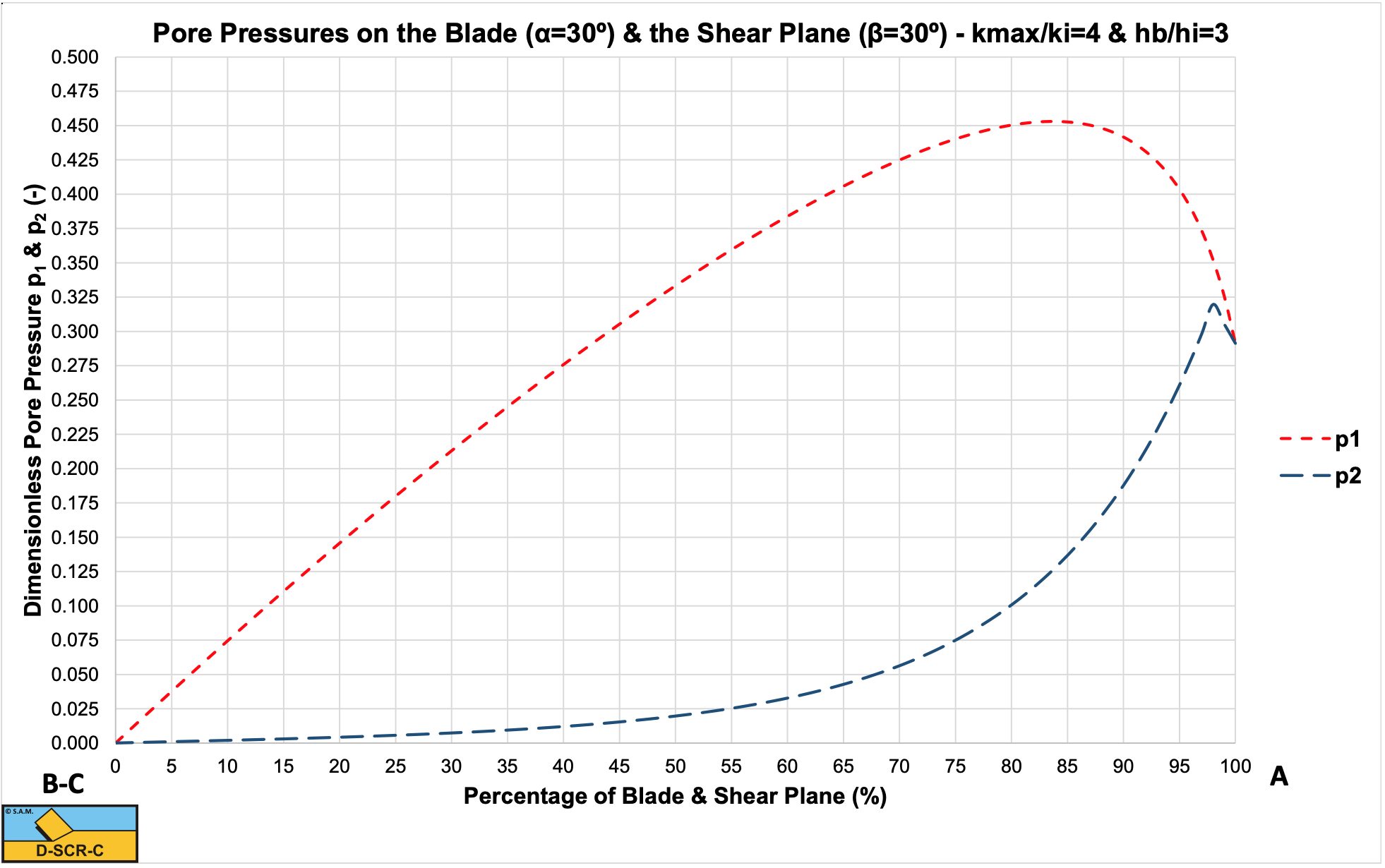
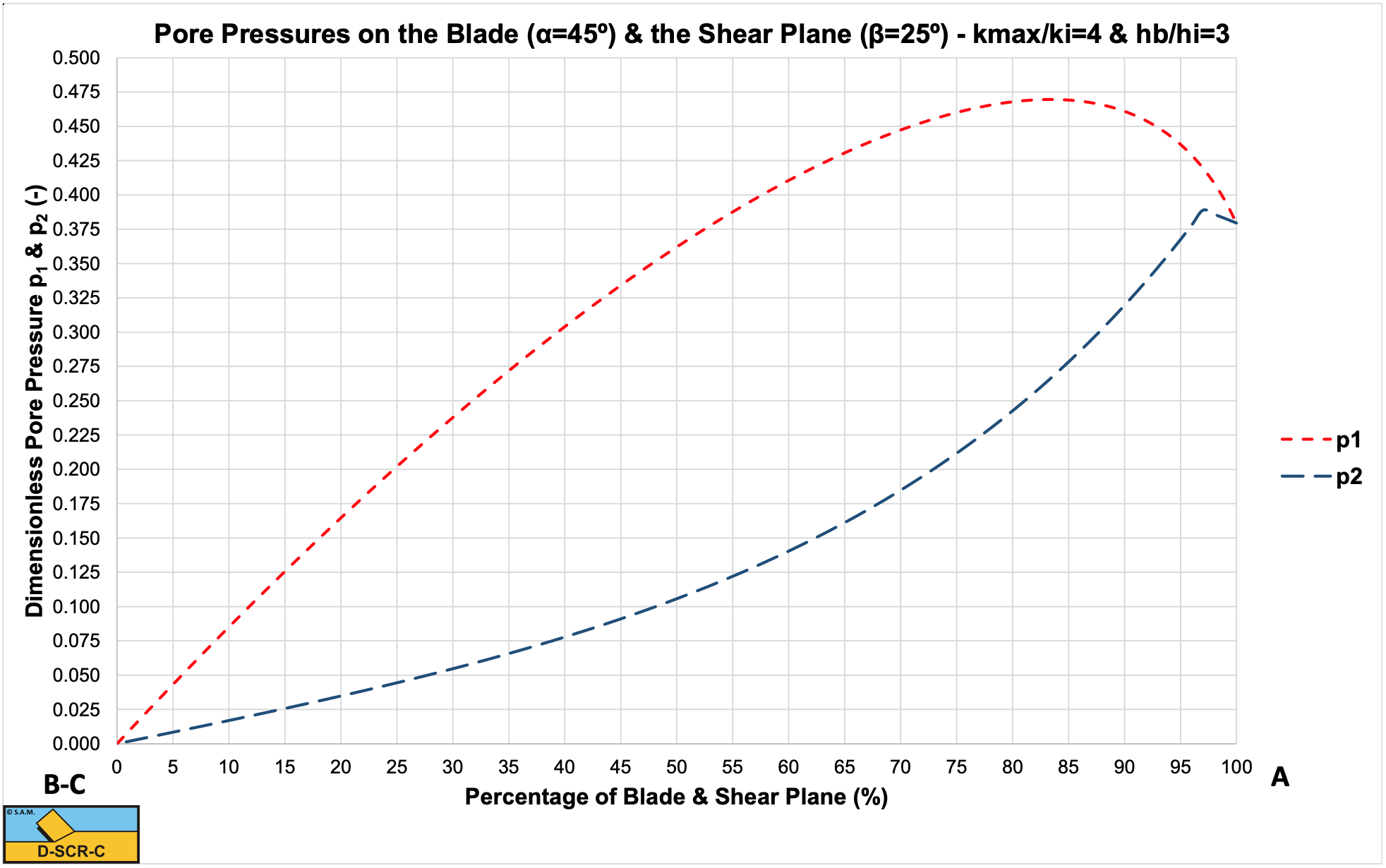
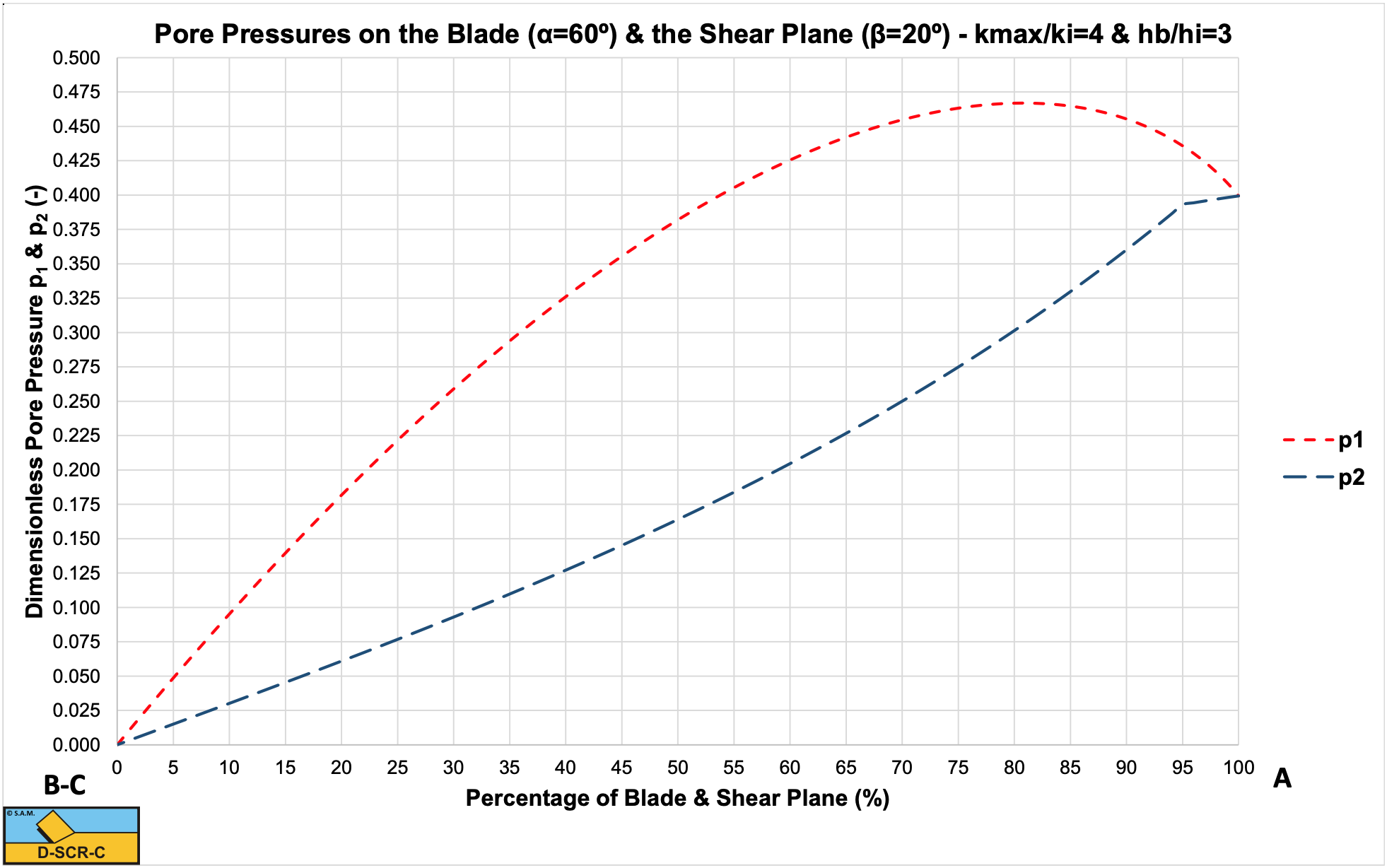
Figure 6-21 shows a program listing to determine the pore pressures with the analytical/numerical method. Figure 6-22, Figure 6-23 and Figure 6-24 show the resulting pore vacuum pressure curves on the shear plane and on the blade for 30, 45 and 60 degree blades with a h_i/h_b ratio of 1/3 and a k_i/k_max ratio of 1/4. The curves match both the FEM calculations and the experiments very well.

Figure 6-23: The dimensionless pressures on the blade and the shear plane, α=45°, β=25°, k_i/k_max=0.25, h_i/h_b=1/2.

Figure 6-24: The dimensionless pressures on the blade and the shear plane, α=60°, β=20°, k_i/k_max=0.25, h_i/h_b=1/1.