5: Integral Boundary Layer Relationships

Boundary layer thickness

The boundary layer thickness, as we have seen, is given by \({\delta}\), and it represents the thickness of the boundary layer measured from the surface to the location where the velocity reaches the freestream value, \({U}\). However, since the velocity within the boundary layer asymptotically approaches \({U}\) it is often difficult to obtain an accurate measure of \({\delta}\). To circumvent this problem the boundary layer thickness can be taken to be when the velocity reaches, say, 1% of \({U}\). As discussed in the last chapter, in a favorable pressure gradient where the pressure decreases along the flow direction,the boundary layer will be thinner when compared with a zero pressure gradient. The additional pressure force in the flow direction increases the local velocity at any given position and the boundary layer reaches the freestream value at a lower value of the cross stream coordinate. This then reduces the boundary layer thickness. The opposite is true for an adverse pressure gradient. Consequently, the boundary layer thickness is directly influenced by the pressure gradient and as such there is a similar impact on the surface stress. A thinner boundary layer caused by a favorable pressure gradient, with the same freestream velocity, will have a larger surface velocity gradient and a higher local surface shear stress.

In general we note that the boundary layer thickness is a function of the downstream coordinate, \(x_{1}\), and \({\delta}\) increases in the \(x{}_{1}\) direction. An alternative way of expressing this is through the Reynolds number, since the Reynolds number depends on \(x_{1} \left ( Re_{x_1}=\frac{\rho Ux_1}{v } \right )\):

\[\delta =f(Re_{x1})\]

Displacement thickness, \({\delta}_{1}\)

The displacement thickness, \({\delta}_{1}\), and momentum thickness, \({\delta}_{2}\), are often used as a measure of the thickness of the boundary layer but are not actually the boundary layer thickness; these two are important parameters in the analysis of the frictional forces on the surface. The displacement thickness is, in general, a function of position, \(x{}_{1}\), along the flow direction as is \({\delta}\). Typically \({\delta}_{1}\) increases with increasing \(x_1\) and is less than \({\delta}\). A sketch illustrating the definition of the displacement thickness is given in Figure 9.1 where \({\delta}_{1}\) is determined based on the mass flow rate within the boundary layer. The velocity distribution can be integrated across the boundary layer, normal to the surface, to determine the mass flow rate at any location, \(x_1\) as

\[\dot{m}=\int^{\delta }_0{\rho u_1dx_2\ S}\label{9.1} \]

where \(u{}_{1}\) is the \(x{}_{1}\) component of the velocity and S is the span, or the distance into the page. The distribution of \(u{}_{1}\) follows the two boundary conditions, \(u{}_{1} = 0\) at the surface and \(u{}_{1} = U\) at the edge of the boundary layer, \({\delta}\).

The surface generated friction by the surface on the flow causes the velocity to decrease at any given \(x{}_{2}\) position along the surface. This decrease across the entire boundary layer results in a decreasing flow rate within the boundary layer with increasing \(x{}_{1}\). Therefore the amount of mass flow lost in the boundary layer due to surface friction can be thought of as local a mass flow deficit. This deficit can be calculated by comparing the actual velocity distribution to the ideal velocity without friction, which would be \({U}\) across the entire boundary layer. The local mass flow deficit at any \(x{}_{2}\) location is then \(d{\dot{m}}_{deficit}=\rho \left(U-u\right)dy\ S\) and the total mass flow deficit is obtained by integrating this across the flow as:

\[\int^{\delta }_0{d{\dot{m}}_{deficit}}={\dot{m}}_{deficit}=\int^{\delta }_0{\rho \left(U-u_1\right)dy\ S}\label{9.2} \]

The mass flow deficit can be equated to mass flow rate loss given as the product of density, \({U}\) and (\({\delta}_{1}\)S), where \({\delta}_{1}\) is an unknown “thickness”. So setting the integral term in Equation \ref{9.2} to this product \(\left ( \rho U\delta_1 S \right )\) and solving for \({\delta}_{1}\) results in:

\[{\delta }_1=\int^{\delta }_{\ 0}{\left(1-\frac{u_1}{U}\right)dy}\label{9.3} \]

which assumes that the density is constant. Equation \ref{9.3} is the definition of the displacement thickness and can be interpreted as follows. If the total mass flow rate lost in the boundary layer due to friction is divided by \(\rho US\) the result is a length that would represent a distance normal to the surface through which all of the lost mass flow rate would pass if it traveled at velocity \(U\)(the velocity it would have if there were no friction.) Another way of looking at this distance is that it represents the vertical distance the surface would need to be moved upward (in the \(x{}_{2}\) direction) to capture all of the lost mass flow rate if the velocity were uniformly at \({U}\), or frictionless. Either of these interpretations indicates that as \({\delta}_{1}\) grows larger along the flow there is an increase in the total mass fow deficit. Since surface friction slows more and more fluid, creating a larger boundary layer thickness in the x direction, then \({\delta}_{1}\) must increase in the downstream \(x{}_{1}\) direction. At any given position along the surface the greater the local surface shear stress the greater the value of \({\delta}_{1}\). Consequently, a favorable pressure gradient which increases the local shear stress compared with zero pressure gradient, results in a larger relative value of displacement thickness.

Momentum thickness, \({\delta}_{2}\)

The momentum thickness, \({\delta}_{2}\), has somewhat of the same interpretation as \({\delta}_{1}\), but it has to do with the momentum rate loss by the frictional forces, rather than the mass flow rate loss. In this case we develop a measure for the momentum rate loss, or momentum deficit, generated by friction. Noting that the momentum rate lost crossing a given vertical plan across the boundary layer is given by:

\[\int^{\delta }_0{\rho u\left(U-u_1\right)dx_2\ S}\label{9.4} \]

where \(\rho udx_2\ S\) is the mass flow rate within an elemental area \(dx_2 S\) w and the expression \(\left(U-u_1\right)\) is the momentum lost per mass flow rate. The product of these two terms integrated over the entire boundary layer \({\delta}\) is the momentum loss rate at any given \(x{}_{1}\) position along the surface. Similar to what was done for the mass flow rate deficit, here we imagine that the momentum rate lost due to friction is equal to the mass flow rate through an area equal to \(\left ( \delta_2S \right )\) with velocity \({U}\) or

\[\rho U{\delta }_2SU=\rho U^2{\delta }_2S=\int^{\delta }_0{\rho u\left(U-u_1\right)dx_2\ S}\]

Dividing through by \(\rho U^2S\) yields the definition of the displacement thickness:

\[{\delta }_2=\int^{\delta }_0{\frac{u}{U}\left(1-\frac{u_1}{U_{\infty }}\right)dx_2}\label{9.5} \]

We can interpret this as the distance \({\delta}_{2}\) the surface would need to be moved in the \(x{}_{2}\) direction into the flow if the velocity is uniformly at \({U}\) in order to reduce the momentum rate equivalent to the actual rate of momentum loss. We can also interpret this somewhat differently as follows.

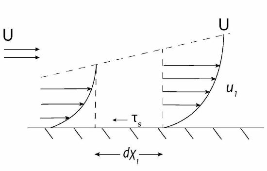
A flat surface is shown in Figure 9.2 indicating the surface shear stress, \({\tau}_{s}\), acting on the fluid. A control volume with an elemental length along the surface, \(x{}_{1}\), and extending upward to the edge of the boundary layer is shown in the figure. The sum of all of the forces acting on the fluid in the control volume consists of \({\tau}_{s}\), since there is zero pressure gradient along the flow, and we assume there is no frictional forces at the top edge of the boundary layer, by definition of the extent of the boundary layer. The momentum equation for this control volume becomes the sum of the forces equal to the change of momentum rate leaving compared to that entering:

\[{-\tau }_sdx_1S={\left(\ \rho U^2{\delta }_2S\right)}_{x+dx_1}-{\left(\ \rho U^2{\delta }_2S\right)}_{dx_1}=\left(\ \rho U^2d{\delta }_2S\right)\label{9.6} \]

where \(d{\delta}_{2}\) is the change of the displacement thickness along d\(x{}_{1}\), while noting that \(\rho U^2S\) is constant along \(x{}_{1}\). The negative sign is included to indicate that the stress on the fluid is in the negative \(x{}_{1}\) direction at the surface. If we rearranging this equation and change the stress to be that on the surface caused by the fluid flow (change the sign of \({\tau }_s\)) then:

\[{\tau }_s=\rho U^2\frac{d{\delta }_2}{dx_1}\label{9.7} \]

Note that this equation is valid for any particular velocity distribution that may exist in the boundary layer. Also, it indicates that the rate of change of the momentum thickness decreases along the flow direction since the surface stress decreases along the flow direction. If one can determine \(\frac{d{\delta }_2}{dx_1}\) it is possible to find the wall surface stress, \({\tau }_s\).

General Integral Boundary Layer Equations

The general integral boundary layer equation is obtained by starting with the Navier- Stokes equation simplified for boundary layer flow:

\[u_1\frac{\partial u_1}{\partial x_1}+u_2\frac{\partial u_1}{\partial x_2}=-\frac{1}{\rho }\frac{\partial P}{\partial x_1}+\nu \frac{{\partial }^2u_1}{\partial x_2}\label{9.8} \]

Note that \(\nu =\frac{\mu }{\rho }\), and is the kinematic viscosity. Since the pressure gradient term can be determined from the freestream flow which is assumed to be inviscid the Euler equation can be used where we ignore gravitational effects such that:

\[-\frac{1}{\rho }\frac{\partial P}{\partial x_1}=U\frac{dU}{dx_1}\label{9.9} \]

Note that body force terms could be included by replacing P with \(P'=P+\rho gh\).

Equation (9.8) is integrated across the boundary layer, in the \(x{}_{2}\) direction, for a given value of \(x{}_{1}\). The boundary conditions for this are no-slip at \(x{}_{2}\) = 0, and u = U at \(x{}_{2} = \delta\). Before we complete this operation we examine the second term on the left hand side in Equation \ref{9.8}. First we use continuity for a two dimensional flow:

\[\frac{\partial u_2}{\partial x_2}=-\frac{\partial u_1}{\partial x_1}\label{9.10} \]

which integrates to:

\[u_2=-\int^{\delta }_0{\frac{\partial u_1}{\partial x_1}dx_2}\label{9.11} \]

and this expression is used in the second term of (9.8). Next each term in Equation \ref{9.8} is integrated from \(y=0\) to \(y=\delta\). For instance the second term becomes:

\[\int_{0}^{\delta}u_2\frac{\partial u_1}{\partial x_2}dx_2=-\int^{\delta }_0{\frac{\partial u_1}{\partial x_2}\left(\int^{x_2}_0{\frac{\partial u_1}{\partial x_1}}dx_2\right)dx_2}\label{9.12} \]

This term is now integrated by parts:

\[\int^2_1{b\ da=ab{|_1}^2-\int^2_1{a\ db}}\]

where we set

\[db=\frac{\partial u_1}{\partial x_1}dx_2, da=\frac{\partial u_1}{\partial x_2}dx_2=\partial u_1\]

The result for this term using the boundary conditions for \(u{}_{1}\) is:

\[-U\int^{\delta }_0{\frac{\partial u_1}{\partial x_1}dx_2}+\int^{\delta }_0{u_1\frac{\partial u_1}{\partial x_1}}dx_2\label{9.13} \]

We insert (9.13) into (9.8) while integrating all other terms and obtain:

\[\int^{\delta }_0{u_1\frac{\partial u_1}{\partial x_1}dx_2}-U\int^{\delta }_0{\frac{\partial u_1}{\partial x_1}dx_2}+\int^{\delta }_0{u_1\frac{\partial u_1}{\partial x_1}}dx_2=\int^{\delta }_0{U\frac{dU}{dx_1}}+\int^{\delta }_0{\nu }\frac{{\partial }^2u_1}{\partial x_2}dx_2\label{9.14} \]

The last term is the viscous term and can be expressed in terms of the shear stress, \(\tau =\mu \frac{\partial u_1}{\partial x_2}\) (the \(x{}_{1}\) derivative of \(u{}_{2}\) is taken to be small compared with the \(x{}_{2}\) derivative of \(u{}_{1}\), consistent with the boundary layer approximations.) So the last term is:

\[\int^{\delta }_0{\nu }\frac

Callstack:
    at (Bookshelves/Civil_Engineering/Intermediate_Fluid_Mechanics_(Liburdy)/05:_Integral_Boundary_Layer_Relationships), /content/body/div/div[2]/p[21]/span, line 1, column 1

We combine the first and third terms of Equation \ref{9.14} as:

\[\int^{\delta }_0{2u_1\frac{\partial u_1}{\partial x_1}dx_2}=\int^{\delta }_0{\frac{\partial \left(u_1u_1\right)}{\partial x_1}dx_2}\label{9.16} \]

Then we rewrite the second term of Equation \ref{9.14} by bringing U inside the integral since it is not a function of \(x_2\), but may be a function of \(x_1\):

\[-U\int^{\delta }_0{\frac{\partial u_1}{\partial x_1}dx_2=\int^{\delta }_0{\left(-\frac{\partial \left(uU\right)}{\partial x_1}+u\frac{\partial U}{\partial x_1}\right)}}dx_2\label{9.17} \]

Getting closer to the final result we combine all these expressions in (9.14) to obtain:

\[\int^{\delta }_0{(\frac{\partial \left(u_1u_1\right)}{\partial x_1}-\frac{\partial \left(u_1U\right)}{\partial x_1}+u_1\frac{dU}{dx_1}}-U\frac{dU}{dx_1})dx_2 = \frac{\tau _s}{\rho }\label{9.18} \]

This is rearrange as:

\[\int^{\delta }_0{\frac{\partial \left(u_1(u_1-U\right)}{\partial x_1}dx_2+\int^{\delta }_0{\frac{dU}{dx_1}}}\left(u_1-U\right)dx_2=-\frac{{\tau }_s}{\rho }\label{9.19} \]

Exchanging the order of integration and derivatives in the first term, changing sign of all the terms, yields:

\[\frac{\partial }{\partial x_1}\int^{\delta }_0{u_1(U-u_1)dx_2}+\frac{dU}{dx_1}\int^{\delta }_0{\left(U-u_1\right)dx_2=}\frac{{\tau }_s}{\rho }\label{9.20} \]

This now allows us to use the definitions of \({\delta}_{1}\) and \({\delta}_{2}\) to arrive at our final form as:

\[\frac{d}{d x_1}\left(U^2{\delta }_2\right)+{\delta }_1U\frac{dU}{dx_1}=\frac{{\tau }_s}{\rho }\label{9.21} \]

We end up with a differential equation in terms of the variables \({\delta}_{1}\) and \({\delta}_{2}\) both of which are functions of \(x{}_{1}\). Recall that U(\(x{}_{1}\)) is determined by the pressure gradient through use of Equation \ref{9.9}, Euler’s equation. When U = constant, as in flow over a flat plate this equation can be simplified to:

(9.22)

where the right hand side is the skin friction coefficient.

The problem of determining the local surface stress distribution is now reduced to Equation \ref{9.21} for flows over surfaces with a pressure gradient or (9.22) for a flat plate with no pressure gradient. Next, we will examine methods to arrive at solutions to this.

Solution Method

There are several methods available to arrive at a solution for Equation \ref{9.21}. We present a typical method that is based on the assumption of a velocity profile in nondimensional form across the flow at any given position, \(x{}_{1}\). The key to this approach is based on the fact that the Blasius solution found a similarity solution and collapsed the velocity profile onto one curve when using proper scaling of the velocity and cross-stream coordinate, the latter also incorporated the stream-wise coordinate to help scale it properly. Here we will assume a non-dimensional velocity profile and use it to determine the integrals in the definitions of \(\delta_2\) and \(\delta_1\).

The proper scaling of the cross-stream coordinate is taken to be the boundary layer thickness, where \({\delta}\) is a function of \(x{}_{1}\) then this scaling combines the cross-stream and stream-wise dependency. We define this new non-dimensional variable as:

\[\eta =\frac{x_2}{\delta }\label{9.23} \]

being careful to note that this variable, \({\eta}\), is not the same as used in the Blasius definition. Next we assume that the nondimensional velocity, \(f=\frac{u_1}{U}\), is some function of \({\eta}\) or:

\[f=f(\eta )\label{9.24} \]

One may say that it is necessary to precisely determine this function since the surface stress, \({\tau}_{s}\), depends on the velocity derivative at the surface. This certainly is the case for the Blasius approach. However, examining Equations (9.21) and (9.22) it can be seen that the surface stress is a function of the integral of the velocity distribution as expressed through the variables \({\delta}_{1}\) and \({\delta}_{2}\). Based on this we conclude that to get a solution we must obtain good values for the integrals expressed in these equations, rather than the surface derivative of the velocity.

Taking this approach it is possible to assume a velocity distribution using the assumed nondimensional form in Equation \ref{9.24} requiring it to satisfy the boundary conditions. One can use this distribution after transforming the integrals in (9.21) into the nondimensional form. We will use the example of flow over a flat plate, governing by Equation \ref{9.22}. This simplifies the details, but the same approach is used for flows with pressure gradients, but requires further input of a known pressure gradient.

First looking at Equation \ref{9.22} written in terms of the skin friction coefficient we have:

\[c_f=2\frac{d{\delta }_2}{dx_1}\label{9.25} \]

We can not evaluate \({\delta_2}\) since we do not know the value of \({\delta}\). We illustrate the process by assuming a polynomial velocity distribution based on Equation \ref{9.24} variables:

\[f=a+b\eta +c{\eta }^2+d{\eta }^3+\label{9.26} \]

There are four parameters in this polynomial, \(a,b,c \text { and } d\) that need to be determined based on boundary conditions on the velocity distribution. Notice that the higher the order of the polynomial the more conditions are needed to evaluate these coefficients. The boundary conditions written in terms of the variables, \(f,{\delta}\) are:

\[f(0)\ =\ 0\]

\[f(1)\ =\ 1\]

\[\frac{\partial f}{\partial \eta }=0\]

\[\frac{{\partial }^2f}{\partial {\eta }^2}=0\]

The last condition is a consequence of all terms in the Navier-Stokes equation becoming zero at the surface if the pressure gradient is zero, and \(u_1=u_2=0\), and then transforming the viscous term into the non-dimensional variables. These four conditions can now be used to determine the four coefficients in Equation \ref{9.26}. The results are:

Inserting these into Equation \ref{9.26} results in the velocity distribution:

\[f=\ \frac{3}{2}\eta -\frac{1}{2}{\eta }^3\label{9.27} \]

This result is unique to the selection of a third order polynomial for the velocity distribution. Next, we rewrite the relationship of \(c{}_{f}\) in terms of the nondimensional variables.

First we define the momentum and displacement thicknesses in terms of \({\delta}\) as:

\[\frac{{\delta }_1}{\delta }=\int^1_0{\left(1-\frac{u_1}{U}\right)d\eta }\label{9.28} \]

\[\frac{{\delta }_2}{\delta }=\int^1_0{\frac{u_1}{U}\left(1-\frac{u_1}{U}\right)d\eta }\label{9.29} \]

Here we have changed the integration from \(dx_2\) to \(d{\eta}\), where \(dx_2=\delta d\eta\) and need to change the limits of the integral accordingly. Notice that once we have an expression for \(f=\frac{u_1}{U}\) from our polynomial, Equation \ref{9.26}, then both \(\frac{{\delta }_1}{\delta }\) and \(\frac{{\delta }_2}{\delta }\) are just constants. The important point now is that we can rewrite Equation \ref{9.25} as:

\[c_f=2\frac{d\delta_2}{dx_1}=2\frac{d}{dx_1}\left ( \left ( \frac{\delta_2}{\delta} \right )\delta \right )=2\left ( \frac{\delta_2}{\delta} \right )\frac{d\delta}{dx_1}\label{9.30} \]

So we have replaced having to know \({\delta}_2 = f(x_1)\) to needing to know \({\delta} = f(x_1)\). We find the latter relationship using our function \(f(\eta)\) as:

\[{\tau }_s=\mu \frac{\partial u_1}{\partial x_2}=\mu \frac{\partial u_1}{\partial \eta }\frac{\partial \eta }{\partial x_2}=\frac{\mu U}{\delta }\frac{\partial f}{\partial \eta }=\frac{\mu U}{\delta }f'(0)\]

\[c_f=\frac{{\tau }_s}{\frac{1}{2}\rho U^2}=2\frac{{\delta }_2}{\delta }\frac{d\delta }{dx_1}=\frac{\mu U}{\delta \frac{1}{2}\rho U^2}f'(0)\label{9.31} \]

This last relationship is a differential equation for \({\delta} = {f(x_1)}\) since \(\frac{{\delta }_2}{\delta }\) and \(f'(0)\) are both constants known from Equation \ref{9.26} using the boundary conditions to obtain Equation \ref{9.27}. Notice that these two constants are dependent on the order of the polynomial selected. Now Equation \ref{9.31} can be integrated to obtain:

(9.32)

where and is a constant dependent on the order of the polynomial selected. Knowing \({\delta = f(x_1)}\) we can find \(\frac{d\delta }{dx_1}\) and then \(c{}_{f}\) using Equation \ref{9.31}. The result is:

(9.33)

For our velocity profile, Equation \ref{9.27} we have: \(\frac{\delta_1}{\delta}=\frac{3}{8}, \frac{\delta_2}{8}=\frac{117}{840}\), and \(f(0)=\frac{3}{2}\). This results in \(C=4.64\) and:

\(C_f=\frac{0.6464}{Re_{x_1}\frac{1}{2}}\)

The overall solution procedure now becomes pretty straight forward: (i) assume a functional form for \(f({\delta})\), (ii) match required boundary conditions to find the coefficients in the equation, (iii) calculate the constant \(\frac{{\delta }_2}{\delta }\), (iv) calculate the constant \(f'(0)\), (v) finally calculate \(c{}_{f}\), which determines the local value of the skin friction coefficient.

To determine the total friction drag force, \(F{}_{D}\), on a surface of length L and area \(A{}_{s}\) = LS one needs to integrate the local surface stress along the distance L. The result is typically written in terms of the overall friction drag coefficient, \(C{}_{f}\) as:

\[C_f=\frac{F_D}{\frac{1}{2}\rho U^2A_s}=\frac{1}{\frac{1}{2}\rho U^2A_s}\int^L_0{{\tau }_sdx_1w}=\frac{1}{L}\int^L_0{c_fdx_1=2c_f(x_1=L)}\label{9.35} \]

where the last designation, \(2c_f(x_1=L)\), means two times the value of the skin friction coefficient evaluated at \(x{}_{1} = L\).

The result assuming the third order polynomial for the non-dimensional velocity profile given above is:

(9.36)

The results when compared with experimental data for the appropriate Reynolds number conditions become very close to these predicted values. Consequently, this procedure is a fairly easy yet surprisingly accurate means to predict friction drag forces on flat surfaces. When pressure gradients come into play, such as surfaces with some degree of curvature it is more of a challenge to obtain a good velocity profile since for this case at the surface the net viscous forces are not zero but are balanced by the pressure gradient. The velocity profiles need to reflect this condition and there are a number of procedures available to address this. The interested reader is encouraged to see F.W. White’s book, Viscous Fluid Flow for some examples.