4: Potential Flow Basics

Continuity Equation

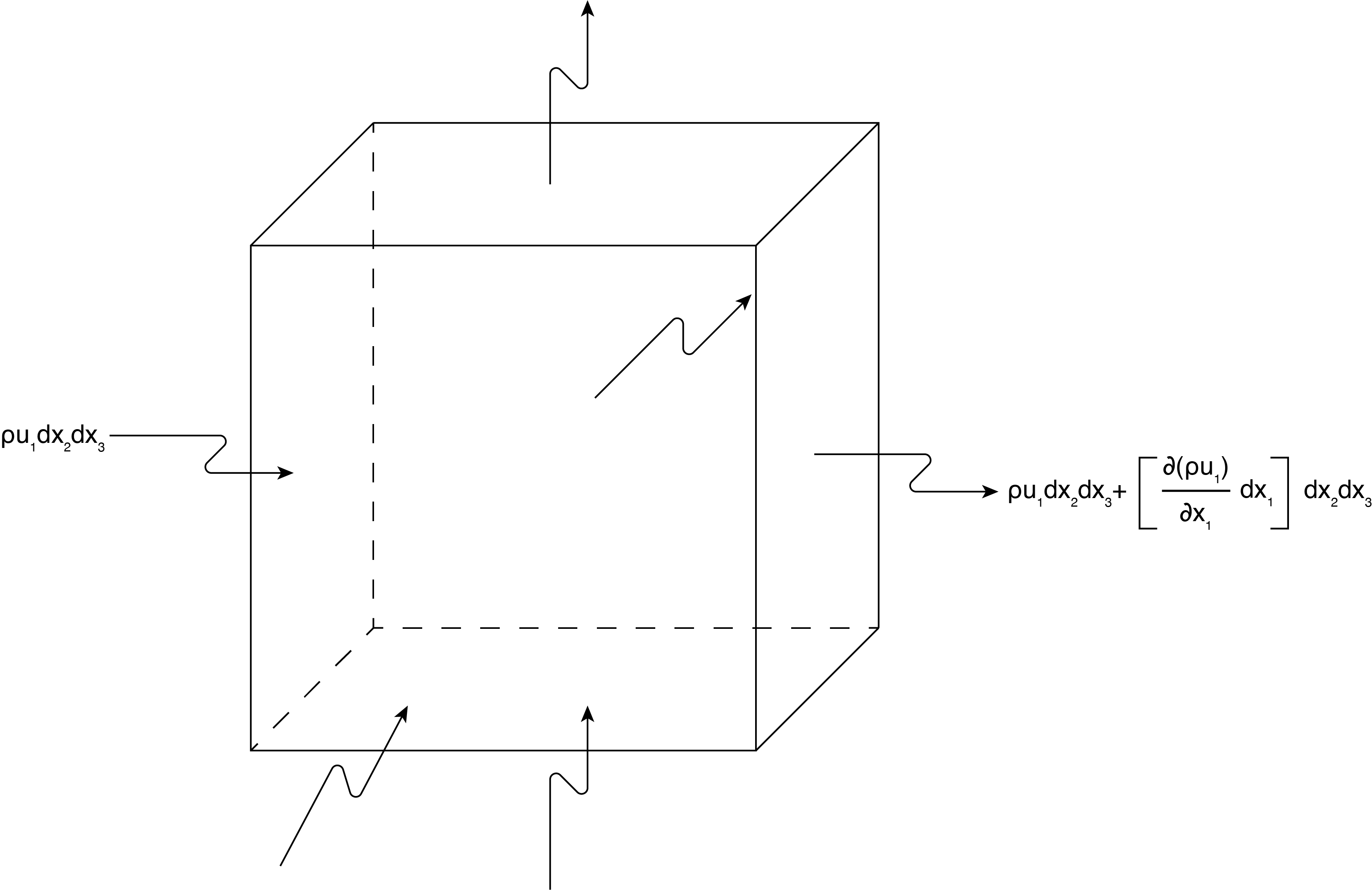
Before we get into describing flows with the velocity potential we introduce the continuity equation. This equation comes from conservation of mass as applied to a continuum of fluid that may be in motion. The basic derivation of the continuity equation is shown in Figure (4.1). Imagine a three dimensional volume in space that for convenience is shaped as a cube. Each face can have mass flow across this geometric element. We are interesting in finding the constraints on the flow field that satisfies conservation of mass for flow in/out of this volume. The basic physics of the relationship that we start from is that no mass can be created or destroyed (thus is conserved) over time. So the net flow in minus the net flow out must be equal to the net change in mass within the volume.

Putting this idea in equation form where the mass flow rate across any specified area for a continuum is the density times the velocity normal to the area times the area. We apply this to the faces of the cube:

Net flow in \({x{}_{1}}\) (outflow minus inflow):

\[{\dot{m}}_{out,x_1}-{\dot{m}}_{in,x_1}=\left[\rho u_1dx_2dx_3+\left(\frac{\partial }{\partial x_1}\left(\rho u_1\right)dx_1\right)dx_2dx_3\right]-\left[\rho u_1dx_2dx_3\right]=\left(\frac{\partial }{\partial x_1}\left(\rho u_1\right)dx_1\right)dx_2dx_3\label{4.2} \]

This is repeated for the \({x{}_{2}}\) and \({x{}_{3}}\) direction where changes of density times velocity are with respect to \(\partial x_2 \mathrm{and}\ \partial x_3\) respectively, and \({u{}_{2}}\) and \({u{}_{3}}\) are used for the velocity, respectively, while using the area \({dx{}_{1}x{}_{3}}\) and \({d{}_{1}xdx{}_{2}}\), respectively. Summing all three of these net flow rates results in a scalar representation of the difference between the outflow and inflow where all possible flow paths in and out are included. Reversing the sign (to make it inflow minus outflow) this must equal to the change of mass within the volume element, \({dx{}_{1}dx{}_{2}dx{}_{3}}\).

This is expressed as:

\[\frac{\partial (\rho )}{\partial t}dx_1dx_2dx_3=-\frac{\partial }{\partial x_1}\left(\rho u_1\right)dx_1dx_2dx_3-\frac{\partial }{\partial x_2}\left(\rho u_2\right)dx_1dx_2dx_3-\frac{\partial }{\partial x_3}\left(\rho u_3\right)dx_1dx_2dx_3\]

or rearranging and dividing each term by \(dx_1dx_2dx_3\):

\[\frac{\partial (\rho )}{\partial t}+\frac{\partial }{\partial x_1}\left(\rho u_1\right)+\frac{\partial }{\partial x_2}\left(\rho u_2\right)+\frac{\partial }{\partial x_3}\left(\rho u_3\right)=0\label{4.3} \]

This is the continuity equation that must be satisfied to conserve mass. Notice that if the flow is steady the first term is zero. Also if the density is constant (incompressible) then the first term, or the partial derivative with respect to time, is zero, and density can be factored from each of the other terms and divided out of the equation. The result is:

\[\frac{\partial u_1}{\partial x_1}+\frac{\partial u_2}{\partial x_2}+\frac{\partial u_3}{\partial x_3}=0=\frac{\partial u_i}{\partial x_i}\label{4.4} \]

where in the last term there is summation by tensor notation. This is the reduced form of continuity for incompressible flow. Notice that this form does not require the flow be steady (even though the unsteady derivative of density is no longer included). The velocity may in fact vary with time.

If we now insert the definition of the velocity potential from Equation \ref{4.1} for each of the velocity components in Equation \ref{4.4} we end up with the following equation for \({\phi}\) for incompressible flow:

\[\frac{{\partial }^2\phi }{\partial {x_1}^2}+\frac{{\partial }^2\phi }{\partial {x_2}^2}+\frac{{\partial }^2\phi }{\partial {x_3}^2}=0\label{4.5} \]

This equation is the Laplace operation on the scalar velocity potential, \({\phi}\), and represents continuity (or conservation of mass) for an incompressible flow.

Before moving on we write the continuity equation using the Material Derivative from Chapter 2. We combine the time derivative of density with the other three terms but notice that there is a difference in the three spatial derivative terms from those found in the Material Derivative, the velocity is included in the derivative in continuity. So if each of these terms is expanded,

\[\frac{\partial \left({\rho u}_i\right)}{\partial x_i}=\rho \frac{\partial \left(u_i\right)}{\partial x_i}+u_i\frac{\partial \left(\rho \right)}{\partial x_i}\]

The we see that:

\[\frac{D\rho }{Dt}+\rho \frac{\partial \left(u_i\right)}{\partial x_i}=0\]

And if the density is \(y\) constant we obtain Equation \ref{4.4} as expected.

Streamfunction

We now introduce the streamfunction, \({\psi}\). This is a scalar quantity as is the velocity potential. For simplicity we will do this in two dimensions, but it is valid in three dimensions as well. Recall we defined a streamline coordinate system (\({s,n}\)) where s is aligned with the velocity vector. In general, for a time dependent flow the streamlines will be continually changing instant by instant. Within a coordinate system (say Cartesian or cylindrical or spherical) the streamline has an equation that can be written out in the selected coordinate system. The equation of this line can be represented by a streamfunction value. This is done as follows.

Consider a line that represents the instantaneous streamline within a flow. In Cartesian coordinates we can write the following for this line where we assume that there is some constant value \(\psi\) associated with the equation for the line:

\[\psi =f(x_1,x_2)=\mathrm{constant}\]

For \(\psi\) being a constant small changes along a streamline we can write:

\[d\ \psi =0=\frac{\partial \psi }{\partial x_1}dx_1+\frac{\partial \psi }{\partial x_2}dx_2\]

\[\frac{dx_2}{dx_1}=-\frac{\frac{\partial \psi }{\partial x_1}}{\frac{\partial \psi }{\partial x_2}}\]

Since \(\frac{dx_2}{dx_1}\) is the slope of the line representing the streamline and since the velocity vector is tangent to the streamline, and the slope of the velocity vector is the ratio of the \({x{}_{2}}\) to \({x{}_{1}}\) velocity components we write:

\[\frac{u_2}{u_1}=-\frac{\frac{\partial \psi }{\partial x_1}}{\frac{\partial \psi }{\partial x_2}}\]

or we can write:

\[u_1=\frac{\partial \psi }{\partial x_2}\ \mathrm{and}\ u_2=-\frac{\partial \psi }{\partial x_1}\label{4.7} \]

Equation \ref{4.7} represents the definition of the scalar \(\psi (x_1,x_2)\) associated with each streamline. If we know expressions for the velocity components as a function of position then we can integrate Equation \ref{4.7} to find the value of the streamfunction, \(\psi\). Similarly if we know the equation for the streamfunction then we can calculate the values of each velocity component through partial differentiation using Equation \ref{4.7}.

Let’s assume an incompressible flow so that the flow field follows the continuity equation given by Equation \ref{4.4}. Now insert for the derivatives of the velocities in terms of the derivatives of the streamfunction. The results is:

\[\frac{{\partial }^2\psi }{\partial x_1\partial x_2}+\frac{{\partial }^2\psi }{\partial x_1\partial x_2}=0\]

This is an identity, in other words it is automatically true, so the existence of the streamfunction, by the given definition, automatically solves the continuity equation. Said another way, if the streamfunction exists by its definition of Equation \ref{4.7} then the flow satisfies continuity for incompressible conditions.

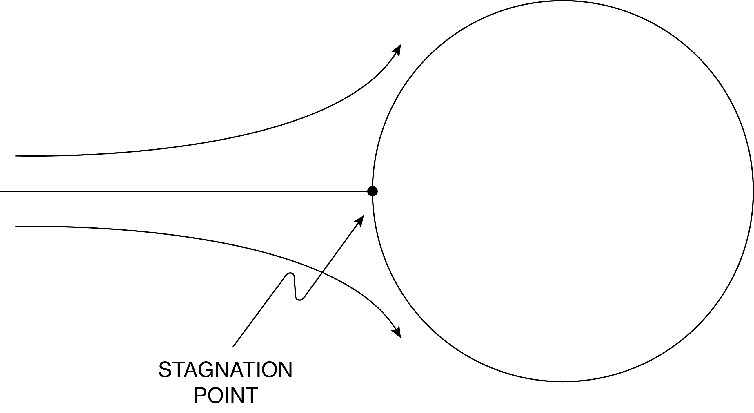
It is possible to take a given velocity field and construct a number of streamlines. At any given point there is a velocity vector and therefor a streamline that passes through it. The only time there can be two or more streamlines passing through a given point (intersecting at some random angle) is if the magnitude of the velocity is zero. Then both partial derivatives of Equation \ref{4.7} are zero and the slope is not defined. A stagnation point is such an intersection of streamlines, as shown in Figure (4.2) for flow over a cylinder. The streamfunction can be continuous up to the stagnation point and beyond, say following the cylinder surface, but it divides at the stagnation point one branch going up and another going down. Stagnation points don’t have to be on surfaces they can be distributed within the flow field.

Streamfunctions are valuable in that they can provide information on local flow rate conditions within a flow field. In general the flow rate (mass or volume) is determined by the velocity vector and an area through which the flow occurs. That is to say, the velocity vector only provides flow rate through an area if there is velocity vector component normal to the area. For a given area we define an outward normal unit vector, \(\hat{n}\) as shown in Figure (4.3). The mass flow rate through the area “A” with this outward normal is given as:

\[\cdot{m} = \rho \boldsymbol{V} \bullet \hat{n}A \label{4.7B} \]

The reader should check the units for this equation. Notice that \(\boldsymbol{V}\cdot \hat{n}\) is the dot product between the velocity and outward normal that results in a scalar whose value represents the projection of the velocity vector in the \(\hat{n}\) direction. To obtain the volume flow rate, \(\dot{Q}\) this expression is divided by mass per volume, or the density:

\[\cdot{Q}=\boldsymbol{V} \bullet \hat{n} A \label{4.8} \]

Now consider a two dimensional steady flow with a streamline distribution as shown in Figure (4.4). Since the velocity vector is tangent to each streamline there can be no flow across a streamline. Consequently, the flow that occurs between two streamlines must remain between those two streamlines along the flow direction. In other words, the flow rate between two streamlines remains constant. The value of the flow rate can be interpreted in terms of the change in the streamfunction value between the two streamlines. This is shown as follows.

Consider the two streamfunctions in Figure (4.4), such that the difference is \(\Delta \psi ={\psi }_2-{\psi }_1\). Next draw, a control volume as shown in the figure, where flow can enter through two areas, \({dx{}_{1}}\) and \({dx{}_{2}}\) (this is two dimensional representation so there is a unit distance into the page). The volumetric flow rate per unit depth into the control volume must balance the volumetric flow rate per unit depth out of the control volume, \(\dot{Q}{'}\).

\[\dot{Q}{'}= \int_{b}^{c}u_2 dx_1 + \int_{c}^{A}u_1 dx_2=u_2\bigtriangleup x_1 + u_1\bigtriangleup x_2\]

\[\dot{Q}{'}= \bigtriangleup\psi_{c-b}+\bigtriangleup\psi_{A-C}=\bigtriangleup\psi_{A-B}=\psi_2-\psi_1\label{4.9} \]

The reason there is a negative sign for \(u_2\Delta x_1\)is that in determining the flow rate between points B and C we integrate along negative \(\Delta x_1\) direction (or the change in \(\Delta x_1\) is negative) Also we have used the definition of the streamfuction, Equation \ref{4.7} to evaluate finite changes, on and . The interpretation then is that the flow rate \(\dot{Q}{'}\) is equivalent to the change in streamfunction value between two points within the flow.

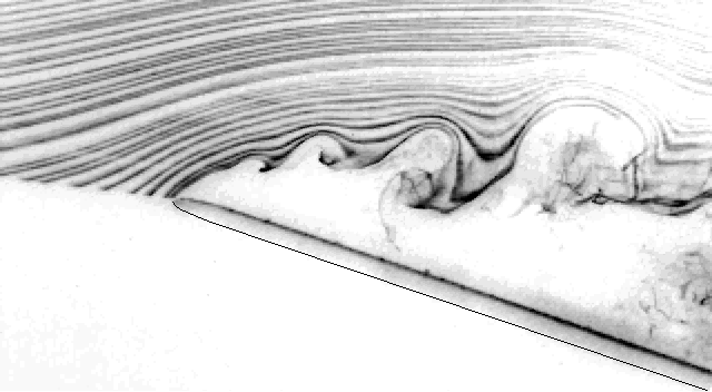
Interestingly, one can use streamline maps to qualitatively and quantitatively evaluate the velocity field. Imagine a wind tunnel test in a two dimensional flow over, say, a wing, as in Figure (4.5). Smoke dye is injected at discrete points upstream separated by some vertical distance between each streamline. The lines of smoke travel downstream and over the wing. As the flow goes over the wing some of the streamlines diverge and some converge (the distance of separation between streamlines changes). Since we have shown that there is constant flow rate between streamlines when the distance between streamlines gets smaller the area of the flow decreases, so the velocity must increase. As streamlines diverge the velocity must decrease. The relationship between cross sectional area and velocity is linear as shown in Equation \ref{4.8}. Measuring the change of distance between adjacent streamlines provides a measure of the amount of increase or decrease of velocity.

We now have a physical as well as mathematical interpretation for the streamfunction. Remember that this is a scalar field function representative of the local velocity. If we use the definition of streamfunction, Equation \ref{4.7} and insert this into the definition of vorticity for a two dimensional flow in the \(x_1-x_2\) plane we obtain the following:

\[{\omega }_3=\left(\frac{\partial u_2}{\partial x_1}-\frac{\partial u_1}{\partial x_2}\right)=\left(-\frac{\partial \psi_2 }{\partial {x_1}^2}-\frac{\partial \psi_2 }{\partial {x_2}^2}\right)=-\left(\frac{\partial \psi_2 }{\partial {x_1}^2}+\frac{\partial \psi_2 }{\partial {x_2}^2}\right)\label{4.10} \]

We see that the vorticity is equal to the negative of the Laplace of the streamfunction (Shown here in two dimensional flow, but is also the case in three dimensional flow). For \({irrotational flow}\) the vorticity is identically zero so:

\[\left(\frac{\partial \psi_2 }{\partial {x_1}^2}+\frac{\partial \psi_2 }{\partial {x_2}^2}\right)=0\]

This shows that the Laplace of the streamfunction is zero for irrotational flow and follows the same results for the velocity potential for incompressible flow. So for irrotational, incompressible (ideal) flow the Laplace of both the velocity potential and streamfunction are equal to zero. This points to the ability to solve the Laplace equation for either of these quantities and from this solution determine the velocity field from the definitions of \(\psi\) and \(\phi\) in teams of the velocity. This will be the approach we take in the next Chapter.

Since both \(\phi \mathrm{\ and}\ \psi\) have the same functional form one might think that they are related to each other. We see this in comparing Equations (4.1) and (4.7), both are related to velocity derivatives. Notice that

\[u_1=\frac{\partial \phi }{\partial x_1}=\frac{\partial \psi }{\partial x_2}\mathrm{\ and}\ u_2=\frac{\partial \phi }{\partial x_2}=-\frac{\partial \psi }{\partial x_1}\]

The velocity is tangent to the constant streamfunction value, but the velocity is normal to the constant velocity potential value. Consequently lines of constant \(\phi\) are normal to lines of constant \(\psi\). It is straight-forward to show that the slope of constant potential lines is \(-\frac{u_1}{u_2}\) while the slope of constant streamfunction lines is \(\frac{u_2}{u_1}\). We will generate plots for specific flows in the next chapter to illustrate this, but shown in Figure 4.6 is an illustration of the orthogonality of the velocity potential lines relative to the streamfunction lines. Velocity is always along the streamfunction line and normal to the potential lines.

In Table 4.1 are the two dimensional expressions in cylindrical coordinates for the various mathematical representations presented here. Note that \({v{}_{r}}\) is the radial velocity component and \({v{}_{r}}\) is the circumferential velocity component. The vorticity only has a z component, as shown, all others are identically zero for a two dimensional flow in \({{r},\Theta}\).

Table 4.1 Cylindrical Coordinate Representation for Incompressible Flow

• Continuity: \(\frac{\partial \left(rv_r\right)}{r\partial r}+\frac{\partial v_{\theta }}{r\partial \theta }=0\)
• Streamfunction: \(v_r=\frac{\partial \psi }{r\partial \theta }\ \ \ \ \ \ \ \ v_{\theta }=\frac{\partial \psi }{\partial r}\)
• Vorticity: \({\omega }_z=\left(\frac{\partial \left(rv_{\theta }\right)}{r\partial r}-\frac{\partial v_r}{r\partial \theta }\right)\)
• Velocity Potential: \(v_r=\frac{\partial \phi }{\partial r} v_{\theta }=\frac{\partial \phi }{r\partial \theta }\)