7: The Panel Method - An Introduction

The panel method is an analysis method that can be used to arrive at an approximate solution for the forces acting on an object in a flow. The method, as we present it here, is based on inviscid flow analysis, so it is limited to the resultant pressure forces over the surface. The panel method is basically a numerical approximation that relies on using discrete elements on the surface of an object and then prescribing a flow element (such as a vortex or doublet or source or sink) on each element that will satisfy certain boundary conditions (like no flow crosses the surface of the object). The interaction of the elements are accounted for and must also satisfy the condition that far from the object the flow should be equal to the free stream velocity approaching the object. There are a number of books and papers written that describe the method in very general terms and even the inclusion of viscous forces to some degree. But here we are just introducing the method to get a feel for its usefulness in external flows, so we will use a simply geometry with a simply distribution of flow elements. More complicated models exist but they all are based on the simplified form presented here.

We will assume that we have potential flow such that the governing equation for the flow field is the Laplace of the velocity potential, \({\mathrm{\nabla }}^2\phi =0\). The boundary condition at an impermeable surface, where the velocity normal to the surface is zero, is \(\mathrm{\nabla }\phi \cdot \boldsymbol{n}=0\). Also, we can put our frame of reference on the object so fluid flow approaches the object. Keep in mind that since it is inviscid there may be a nonzero velocity component tangent to the surface. Also, the goal is to determine the velocity on the surface, and once this is found the Bernoulli equation can be used to find the local pressure distribution. The pressure can then be integrated over the surface to find the force by the fluid flow.

Without deriving this it can be shown that the following defines the velocity potential at any point P in the flow field (using Green’s Identify):

\[\phi \left (P \right)=\frac{1}{4\pi }\int{(\frac{\mathrm{\nabla }\phi }{r}-\phi \mathrm{\nabla }\frac{1}{r})\cdot ndS}\label{6.1} \]

where the integral is over the surface area of the flow (assuming two dimensional flow), S. This equation indicates that to solve for the velocity potential we must evaluate the integral on the flow boundaries (both the solid surface and infinitely far away).

This can be shown to be a result of the application of the divergence theorem that says:

\[\int{n_ju_jdS}=\int{\frac{\partial u_i}{\partial x_i}d\forall }\label{6.2} \]

where \({u{}_{i}}\) is the velocity vector. This states that the rate of expansion of a volume of fluid, given by the divergence of the velocity vector, within a given volume equals the flux through the volume boundaries. If the fluid is incompressible then the right side is zero and the net flux through the entire boundary is zero (this is the general argument for the conservation of mass of steady flow).

All this is nice and can be a powerful tool to find \(\phi\) and therefore the velocity in the flow. But we really don’t need to find the potential of the entire flow, what our goal is, is to set up a flow that we know satisfies the velocity boundary condition at the surface of the object (with no velocity component across the surface) and far from the surface where the velocity is known to be the freestream velocity. Once this is established the force can be found. That is to say we only need to evaluate the surface velocity and then the pressure on the surface.

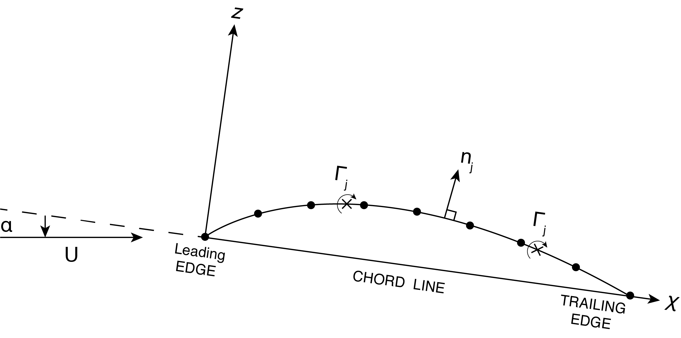
The general approach is to select a “grid” which is a series of “panels” that form the surface. Here we take the panels as straight flat surfaces arranged over the real surface. In the limit of very small panels the constructed surface will simulate the actual surface. On each panel we place a distribution of flow elements (like sources, sinks, vortices, etc) that when combined together will result in a flow field that will satisfy the surface boundary condition. There are lots of ways to identify which elements to use and how they may be distributed on the panels. Here we will use vortex elements, with one placed on each panel. The net flow is the result of superposition of the flow set up by each vortex on each panel element. So at each point in the field we add together the flow caused by all of the panel elements using the superposition rule. The panels that are far away from a given point will have less and less influence on the flow because the strength of the flow caused by a flow element decreases with distance from the element origin. For instance for a “source” the velocity decreases with increasing radial position because the flow is spreading out away from the source. But the influence never really goes to zero.

In placing a series of panels over the surface we first need to specify the size of each panel. We place a vortex of some strength some where on the panel (whose location is shown below) and we must identify points on the surface where we want to make sure that the velocity is zero across the surface. To be clear, individual points on each panel are used to evaluate the element (vortex) flow field –it needs its own origin, or coordinate system, to write an equation for the flow generated by this element. We also only pick a point on the panel to check to make sure that the net sum of contributions from all elements results in zero flow across the surface. The fact that we only satisfy the condition at one point on each panel will be satisfactory if the panels are made to be reasonably small. These points are called “collocation points” on each panel. In the end each panel will have coordinates that define its location on the surface, coordinates for the element location on the surface and coordinates for the collocation point.

The method of solution for the force on the object is the determination of the magnitudes or strengths of the elements on each panel. Once we have this distribution of strengths we can calculate the total lift on the surface that results from all of these elements. Recall that the lift experienced by a surface is really the component of the pressure at the surface integrated over the surface area in a direction normal to the approach velocity vector of the flow — it is not necessarily vertical, but normal to the freestream velocity.

For illustration we are going to use flat plate panels with vortex elements, one per panel. To get an idea of how to define the vortex origins on each panel we can examine flow over a single flat plate at some angle of attack to the freestream velocity vector, \(\alpha\).

First we define the “center of pressure”, \({x{}_{cp}}\). This is the location on the surface where the resultant lift force caused by the distributed load on the surface acts such that there is no net moment on the surface (see F.M. White, Chapt. 8, for some details on this). In general, if the moment on the surface about the leading edge is \({Mo}\), and \({L}\) is the lift force then using \({x}\) as the coordinate measured along the flat surface from the leading edge then:

.

Consider now flow over the same flat surface, the lift we have seen is \(L= \rho {U} \Gamma\) note that we are going to define \(\Gamma\) as positive clockwise — this is opposite to what we have done previously, but it helps get rid of some negative signs, this is not necessary, but convenient. To find out the value of \({x{}_{cp}}\) we use the theoretical evaluation of the lift force based on “thin airfoil theory”. The interested reader can refer to F.M. White Chapt. 8 for details on this. First, assuming a two dimensional flow, we assume that there is some continuous distribution of vorticity over the surface (in contrast to discrete vortex elements), such that there is a local circulation per unit length of surface, \({\gamma (x)}\). The surface integral of this distribution results in the net total circulation: \(\mathrm{\Gamma }=\int^c_0{\gamma dx}\) where “c” is the length of the flat surface, which we call the “chord”.

The Kutta condition is imposed where we want the flow to leave the surface flowing parallel with the back (trailing) edge. If this is a surface like an airfoil we want both the top and bottom flows to leave smoothly from the trailing edge. For this to happen then we don’t expect there to be a pressure difference between the top and bottom of the surface at the trailing edge, which would cause the flow to deflect up or down. If there is no velocity or pressure difference across the flow at the trailing edge the local circulation at the trailing edge, \({(x=c)}\), must be zero. So now we have a boundary condition for the integration of \({\gamma (x)}\) to get the total circulation \(\Gamma\), that is \({\gamma = 0}\) at \({x=c}\). The needed distribution has been figured out for a single flat surface at an angle of attack of \(\alpha\), the angle between the oncoming flow and the surface. The function that works is: . The integral of this expression for \({\gamma(x)}\) yields the value of \(\Gamma\). Once the circulation is known then the lift, \({L,}\) can be found. Using this lift, and also using the above definition of \({x{}_{cp}}\), it turns out that the “center of pressure occurs at . So by assuming the lift force occurs at \({x{}_{cp}}\) then there is no moment caused by the distributed pressure force.

The lift force, \({L}\), as calculated as stated above, can be made nondimensional by divided by , where b is the span of the surface (in and out of the page). The result is an expression for the lift coefficient:

\[C{}_{L} = 2 \pi \sin \alpha\label{6.3} \]

This result is the thin airfoil theory result for the lift on a surface at angle of attack, \(\alpha\). So at this point, we take this result for a flat surface and place vortex elements at the center of pressure for each flat element, which will be at a point ¼ of the distance along the panel from the beginning edge of the panel. Although this is not absolutely required for the panel method it is a convenient choice. As panel size is reduced smaller and smaller the impact of this choice becomes small.

The next step is to find the location where we want to impose the condition of zero velocity crossing the surface for each panel. For this we are using a coordinate system for the panel to be (\({x,z}\)) where \({x}\) is, again, along the flat surface from the panel leading edge and \({z}\) is normal (upward) from the surface. To find these collocation points, we note that the the velocity set up by a vortex element at location \({r}\) from the origin is . Writing this in Cartesian coordinates where at the panel surface \(v_{\theta }=\ w\) (where \({w}\) is the \({z}\) component of velocity) is:

\[w=-\frac{\Gamma }{2\pi }\frac{(x-x_o)}{{(z-z_o)}^2+{(x-x_o)}^2}\label{6.4} \]

where \((x_o,z_o)\) is taken as the center of pressure (where the vortex element is located). Also, since the collocation point is on the surface then both \({z}\) and \(z{}_{o}\) are zero.

To get the total normal component velocity at the panel surface we add together \({w}\) being the velocity normal to the surface induced by the vortex, with the component of the freestream flow normal to the surface which is at angle \({\alpha}\) to the surface, \(U \sin \alpha\), and set this to zero:

\[w+U\ sin\ \alpha =0\label{6.5} \]

We next insert Equation \ref{6.4} for \({w}\), with \({z{}_{o} = 0}\) and . And we define the location at which we evaluate the zero normal velocity component as the collocation point as: \({x= kc}\). Finally we solve for “\({k}\)” to be . This says that the \({x}\) location along any given panel where the boundary condition is to be satisfied is at . Recall that the vortex element is located at .

In summary, once the panels are set up on the surface, each has its own angle of attack, \(\alpha_{\rho}\), depending on the local orientation of the surface. Each panel has a vortex element located at its own center of pressure and the normal velocity must be equal to zero at measured from the front of each panel. An equation can be written for the zero velocity condition at the collocation point of a panel by taking the sum of all of the contributions from all of the panels, each with a different vortex strength \(\Gamma_{\rho}\), and setting this sum to zero. This will result in N equations (one for each panel) with N unknowns for \(\Gamma_{\rho}\) for each panel. We can then solve for all \(\Gamma_{\rho}\) using this set of equations.

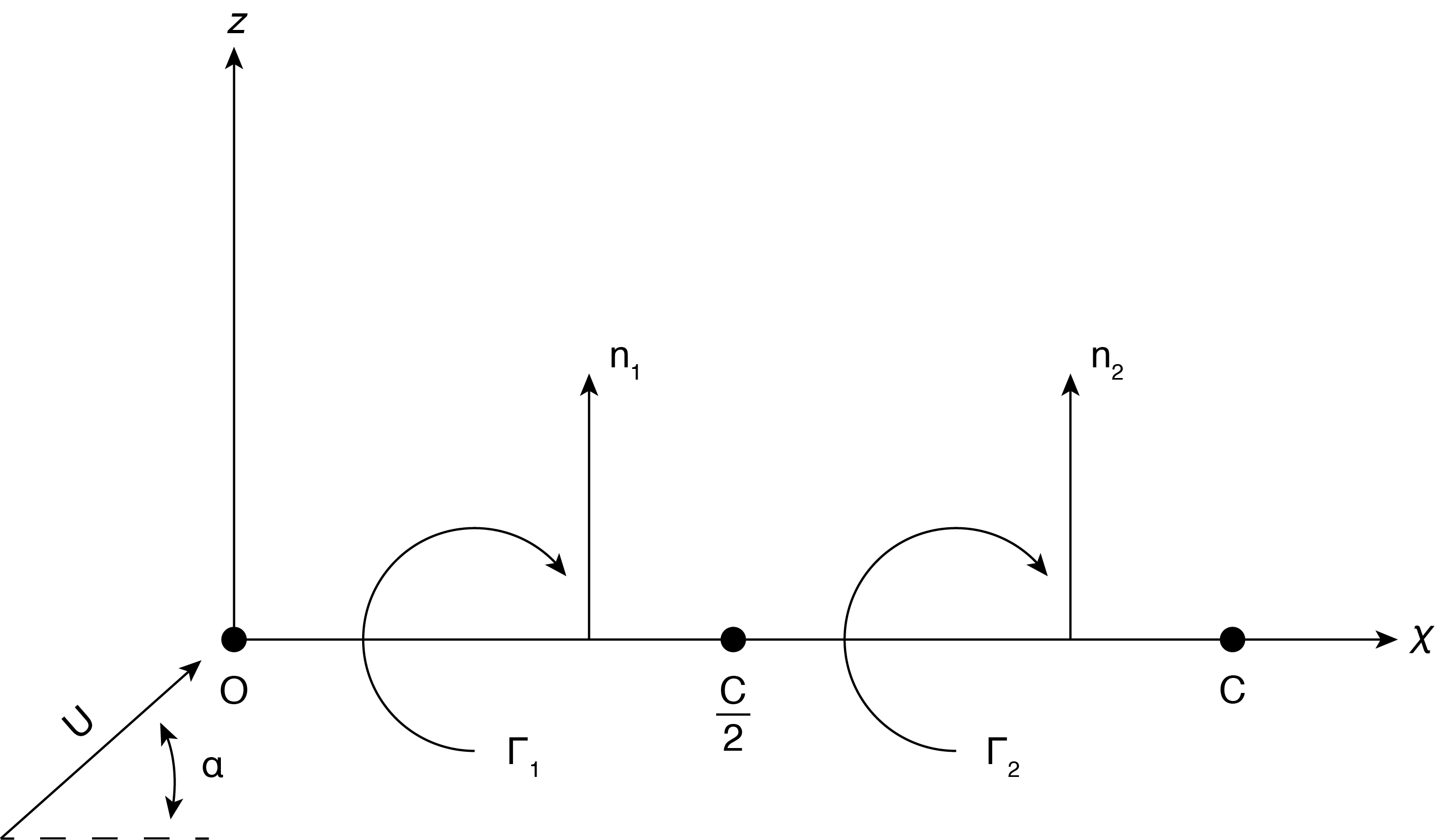
Now we can set this up for a simple example to help pull all of this together, see Figure 6.3. We use a thin flat surface representing a flat airfoil at an angle of attack of \(\alpha\), with a uniform approaching flow of U. We use two panels for illustration. Note that the entire length of the two panels together is “c”, NOT the length of each panel. Also, \({x}\) and \({z,}\) used previously for a single panel, are along and normal to a line from the start to the end of the surface, respectively. This provides a coordinate system for the “system” of panels. For this simple case the angle of attack for both panels are the same, but we allow individual panel vortex strengths, \({\Gamma}_{1}\) and \({\Gamma}_{2}\).

In determining the vortex location for each panel, using the overall coordinate system we get (c/8,0) and (5c/8,0) for panel 1 and panel 2, respectively. The collocation points are (3c/8,0) and (7c/8,0), respectively.

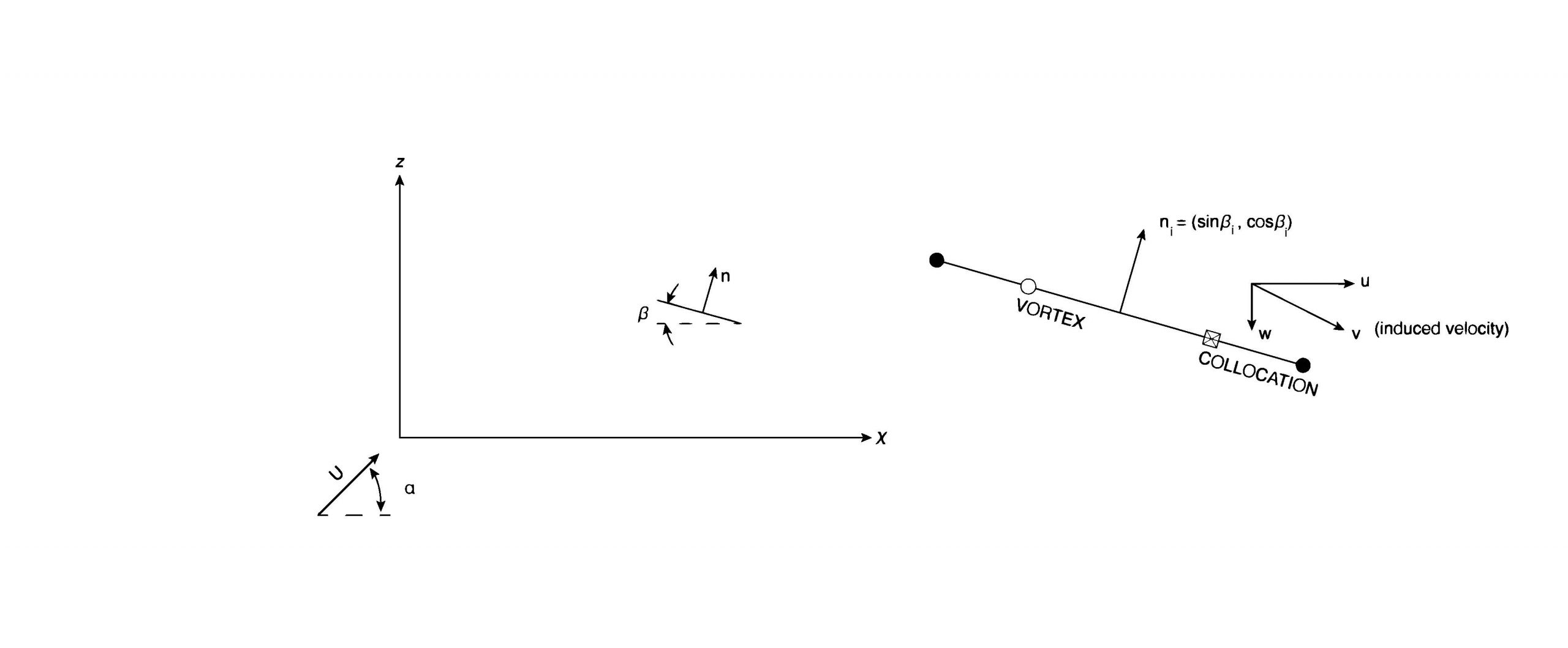
Note that the each outward normal, \(n_{i}\), points in the same direction for this case since both panels have the same orientation, but in general each panel could be at some angle \(\beta_{i}\). Figure 6.4 shows the general definition of the panel angle to the chord, the latter being along the \({x}\) axis. The outward normal to the panel is given as \(n_{i}\). For the general case shown in Figure 6.4 the outward normal is at an angle \(\beta_{i}\) to the \({z}\) axis.

The general equation for the boundary condition is Equation \ref{6.5}, which we write slightly differently as:

\[v_i\cdot n_i=-U\cdot n_i\label{6.6} \]

Where \(v_i\) is the induced velocity by the set of vorticies evaluated at each panel \(j\) and \(n_i\) is the panel outward normal. The left hand side is the dot product of the induced velocity with the outward normal. The right hand side is the component of the freestream velocity aligned with the outward normal. These two balance each other to yield zero velocity crossing the panel. The induced flow from all of the panel elements needs to be added together to get the value of \(v_{i}\) in the above equation.

The general form for the velocity, which has components identified as \({u,w}\),at any point in the flow with a vortex element located at (\(x_o\), \(z_o\)) is obtained from above and written here as:

\[u=\frac{\mathrm{\Gamma }}{2\pi }\frac{(z-z_o)}{{(x-x_o)}^2+{(z-z_o)}^2}\label{6.7} \]

\[w=\frac{\mathrm{-}\mathrm{\Gamma }}{2\pi }\frac{(x-x_o)}{{(x-x_o)}^2+{(z-z_o)}^2}\label{6.8} \]

where we have transformed \(v_{\theta }\) into the Cartesian components \({u,w}\).

Writing this as a matrix we obtain a general expression for the induced velocity anywhere in the flow \(\left ( x, z \right )\):

\[\binom{u}{w}= \frac{\Gamma}{2 \pi r^2} \Big ( \frac{01}{-10} \Big ) \binom{x-x_o}{z-z_o}\label{6.9} \]

Note here that \(x-x_o\) is the distance along the x axis from a vortex element to the point of interest where the velocity is being evaluated. Similarly for \({{z-}z_o}\). Since the values for \(\Gamma\) are not known, it is convenient to write this set of two equations for a “unit value” of \(\Gamma\), that is \(\Gamma=1\). Keep in mind that the flow caused by each vortex when evaluated on a surface results only in a component normal to the surface. We also are going to use values of \(x_{o}\) and \({x}\) based on the location of the vortices and collocation points, respectively.

Consequently, for our two panel example, where each panel is along the chord line, or the \({x}\) axis, we can write the velocity components given below, however here these velocities assume \({\Gamma}=1\) in the above equations. The notation used below is that the first subscript, \({i}\), represents the collocation point of interest at some panel, and the second subscript, \({j}\), identifies the vortex element at some panel that induces the velocity at the \({i}\) collocation point. That is to say these subscripts do NOT represent components of vectors in space in the conventional manner, and here \(u\) and \(w\) are the \(x\) and \(z\) component of the velocity at the surface.

\[(u_{11}, w_{11}) = \left (0, -\frac{1}{\frac{2 \pi c}4} \right ) = (0, -\frac{2}{\pi c})\label{6.10} \]

\[(u_{21}, w_{21}) = \left (0, -\frac{1}{\frac{2 \pi 3 c}4} \right ) = (0, -\frac{2}{3 \pi c})\label{6.11} \]

\[(u_{12}, w_{12}) = \left ( 0, \frac{2}{\pi{c}} \right )\label{6.12} \]

\[(u_{22}, w_{22}) = \left ( 0, - \frac{2}{\pi{c}} \right )\label{6.13} \]

For instance, \(u_{12}\) is the \({x }\) component of velocity at the collocation point of panel 1 caused by the vortex element on panel 2. Also, \(w_{12}\) is the z component of velocity at collacation point 1 caused by the vortex element on panel 2.

We can define, again for \(\Gamma_{\rho} = {1}\), for each panel with vortex \({j}\), the following matrix \(a_{ij}\):

\[a_{ij}={\boldsymbol{v}}_{ij}\cdot \boldsymbol{n}\label{6.14} \]

This represents the component of the induced velocity in the outward normal direction for a given panel \(\Gamma=1\). We need to be careful here with this notation, \({v}_{ij}\) in the equation above is the velocity vector caused by the vorticies with unit value circulation with the subscripts: \({i}\) represents the collocation point and \({j}\) the vortex location inducing that flow. Also, the dot product with \({n}\) (the outward normal for each panel), gives the projection of \({v}\) normal to the surface. For example for the above example \(n\) is only in the \(z\) direction.

\[a_{11} =\left ( 0, - \frac{2}{\pi c} \right ) \cdot (0.1)=-\frac{2}{\pi c}\label{6.15} \]

so the elements \(a _{ij}\) are quantities representing a measure of the velocity contribution normal to each panel from each vortex \({j}\) at each collocation point \({i}\) for a \(\Gamma_{j}=1\) at each panel.

Once we have identified the components \(a_{ij}\), which, as shown above for the two panel example, are determined only by geometry, it is possible to use the impervious boundary condition to find each of the values for \(\Gamma _{j}\). We have a general equation for our two element surface for panels \({i}=1,2\) that says the sum of the outward normal velocity at each panel with the freestream component normal to that panel must be zero. The outward normal velocity due to summation of the induced velocity over both panels is for some unknown distribution of circulations, \(\Gamma_{j}\):

\[\sum^2_{j=1}{a_{ij\ }{\mathrm{\Gamma }}_j}\label{6.16} \]

So this expression is balanced by the contribution from the free stream velocity: \(-U\cdot n\) (this is the component of U normal to the surface).

The final system of equations become:

\[\sum^2_{j=1}{a_{ij}{\mathrm{\Gamma }}_j=-(U_x,U_z)\cdot (n_x,\ n_z)}\label{6.17} \]

Here the right hand side value of \({U}\) is represented as the vector (\({U}_{x},{U}_{z}\)) indicating that \({U}\) is a vector with \({x}\) and \({z}\) components that depends on the angle of attack given by the chord line. The \({x,z}\) components of the outward normal will depend on the angle \({\beta}\) for each panel. The geometry of all of the panels fully determines \(a_{ij}\), as shown above in the simple two panel example. Consequently, once the geometry is known the values of \(a_{ij}\) and \((n_x,\ n_z)\) are all determined. Then knowing \({U}\) the set of Equations (6.17) provides the means to find all of the values of \({\Gamma_j}\), where the index represents each of the panel vortices. In the above two panel example there are two values of \({\Gamma}\).

From the solution of \(\Gamma_j\) we can find the lift on each panel, \(\Delta L_j=\rho U \Gamma_j\) and then the total lift as the sum over all panels:

(6.18)

Recall that the lift is normal to the direction of the freestream velocity, so the lift of each panel, even though the panels may all be at different angles of attack, are all in the same direction.

It is also possible at this point to calculate the velocity tangent to the surface at each panel. That is to say, instead of finding the component normal to the surface to satisfy the impermeable boundary condition find the component tangent to the panel, for each panel and combine this with the component of U tangent to the panel. The induced velocity tangent to the panel can be found using the dot product of the vortex induced velocity with the unit vector tangent to the panel. The tangent unit vector is given by its \(x\) and \(z\) components as \(cos\beta_i\), \(sin\beta_i\), respectively with \(\beta_i\) being the angle of the panel relative to the chord line which is the \(x\) axis, show in Fig 6.4. The freestream contribution is found from the value of U. This combined velocity yields the velocity vector of the flow at each panel and can be used in the Bernoulli equation to find the pressure at each panel. The Bernoulli equation is applied from a known upstream condition (known pressure and freestream velocity) to each panel in order to calculate the panel pressure.

Thin Airfoil Theory Overview

This is an overview of what is known as “Thin Airfoil Theory” used to develop some major results used to analysis flow over airfoils in general, and provide insight into the nature and trends of lift forces generated by flow over airfoils. Airfoils in general come in different geometries and shapes that induce flow perturbations on an approaching flow. These perturbations to the velocity field result in pressure changes that cause a net force on the foil. The force is typically divided into the component aligned with the oncoming flow direction of the fluid (drag force) and the force normal to the oncoming flow direction, (lift force). Viscous effects are not included, but the interested reader may explore some of the options of how certain viscous effects are included by researching on the internet (for instance J.E. Yates, 1980, “Viscous Thin Airfoil Theory”, Aeronautical Research Associates of Princeton, Report 413, as well as several more recent developments). In this short description we are limited to mostly two-dimensional steady flow, although the theory can be extended. Thin airfoil theory can also be extended to unsteady flows such as vibrating or oscillating foils or rotating airfoils (see J. Katz and A. Plotkin, 2010, Low Speed Aerodynamics, Cambridge University Press,).

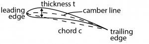
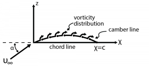
The designation of a “thin” foil provides several mathematical conveniences, which includes the use of “small perturbations” to the freestream flow. This allows some simplification of terms in the governing equations. These mathematical details are not discussed here, but are available in more advanced book on aerodynamics (see J. Katz and A. Plotkin, Low Speed Aerodynamics) The geometric terms used to define the geometry of an airfoil are shown in Figure 6.5. The assumption is that the foil thickness (its maximum value) is much less than the chord length, \(c\), of the foil. The chord length is measured from the leading edge to the trailing edge (in a straight line called the chord line) of the foil. The leading edge is at the front tip and trailing edge is at the rear tip. This can be seen in the figure below which shows the chord length, thickness and also the “camber line” for a given cross section of a wing. The camber line is a line extending from the leading edge to trailing edge that defines the mid-point between the top and bottom of the foil and its effects are discussed later. The degree to which this is curved (rather than falling directly on top of the chord line) defines the “camber”.

The general flow situation needed to generate a lift force involves asymmetry between the flow above and below the foil. As flow goes over and under the foil (from the left in the figure), due to asymmetry the flow over the top will be different from that on the bottom. Asymmetry can be set up in two ways, one by foil shape and the other by rotating the foil relative to the freestream flow direction. If the chord line is curved upward providing camber (see figure) then the flow path along the top and bottom will be different and the velocities most likely will differ. The other way to create asymmetry is to tilt the foil relative to the flow of the fluid, \(U\), this tilt is called the angle of attack, \(\alpha\). Specifically, the angle \(\alpha\) is between the chord line and the freestream velocity. The velocity difference between the top and bottom flow will imply that the pressure distribution along the top and bottom are also different from each other. A net force results acting on the foil by this pressure difference. Integrating the pressure difference along the entire foil yields the net force.

In thin airfoil theory, typically an inviscid flow is assumed (no consideration of frictional force between the flow and the foil). However, viscous forces occur at the foil surface and are assumed to result in vorticity perturbations along the surface. The foil thickness is taken as thin so the top and bottom surfaces are taken together as a single surface with flow over the top and bottom along the camber line. The flow is analyzed using a distribution of local vorticity placed along the camber line. This is called a vortex sheet (in that it extends into the span of the foil) and is shown in Figure 6.6. as a series of small vortices distributed along the foil from leading edge to trailing edge. We denote this distribution by \(\gamma (x)\) which represents the local circulation per length \(dx\). Recall circulation has units of velocity times distance (m2/s), so \(\gamma(x)\) has units of (m/s). Note that \(\gamma (x)\) is not a constant along the foil. For this analysis we assume that circulation is positive if rotation is clockwise. This is opposite to the more conventional sign for circulation previously used, but this change is convenient for airfoils since this designation allows for the generation of upward lift for positive circulation.

General Formulation of Coefficient of Lift

The flow over the foil in reality is viscous flow and it forms a viscous layer of flow (a boundary layer) along the foil. Within this thin layer is vorticity based on the local magnitude of the velocity derivative, , where \(y\) is the coordinate normal to the foil surface. As was mentioned, this distribution of vorticity gives rise to the local circulation distribution \(\gamma(x)\). Also, the integration of \(\gamma(x)\) along the entire foil results in a value of total circulation for the foil, \(\Gamma\), such that:

\[\Gamma=\ \int_{0}^{c}\gamma\left(x\right)dx\]

Because the foil is a solid surface with no flow across it. Then we know that the circulation set up in the boundary layer is not able to cause flow into the foil, rather by superposition, the sum of the flow induced by the local vortex flow, \(dv_v\), determined by the magnitude of \(\gamma\)(x), must be balanced by the freestream flow component normal to the foil surface (which is at angle \(\alpha\) to the freestream if we neglect the small camber for now). Since these two velocities must balance yielding no flow across the foil, then the vortex induced velocity can be written as:

\[dv_v = U\sin \alpha\]

Note that the vortex induced velocity is given by \(\gamma (x)dx = 2 \pi r dv_v\), where \(r\) is the distance from the center of the vortex to some point along the foil surface. To get the entire induced velocity integration is required along the entire foil chord length, c. This can be expressed, for a flat airfoil at an angle of attack of \(\alpha\) as:

\[\int_{0}^{c}{dv_v=\int_{0}^{c}{\frac{\gamma(x)}{2\pi r}dx}}\]

The above integral would need to be evaluated along the foil containing a line distribution of vortices given by \(\gamma\)(x) to find the induced velocity at any point on the foil. To do this the variable position “r” needs to be expressed in terms of the coordinate \(x\), measured along the chord line. If we select a position on the foil, \(x_o\), that designated a given location of a vortex sheet element then \(r = (x_o – x)\). Using the above expression for \(dv_v\) in terms of \(U \sin \alpha\) we obtain an integral equation for the distribution of local circulation:

\[U\sin{\alpha}=\ \int_{0}^{c}{\frac{\gamma(x)}{2\pi(x_o−x)}dx}\label{6.19} \]

The above condition needs to be satisfied for the given distribution \(\gamma(x)\) along the foil. However, we need a boundary condition at \(x = c\) that specifies \(\gamma(c)\). This is done by introducing what is known as the Kutta Condition. This is based on the observed flow condition at the trailing edge of the foil, assuming the geometry is such that the flow from the top and bottom sides meet at a point (the trailing edge) and that flow exits the foil “smoothly” from the top and bottom surfaces such that there is no vorticity as the flow leaves the trailing edge. Physically this would occur if there is no roll-up of the flow say from the bottom to the top surface. If the velocities on top and bottom at the trailing edge are identical, then the pressures are identical by the Bernoulli equation, and the flow has no tendency to swirl. So, this condition is expressed as \(\gamma(x=c) = 0\). It can then be shown that the integration in Equation \ref{6.19} is found to satisfy the Kutta Condition for the following distribution of the vortex sheet:

(6.20)

(See the extra comments on the Kutta condition below)

With this distribution of \(\gamma(x)\) the total circulation, \(\Gamma\), can be determined. Note that this value of \(\Gamma\) depends on the angle of attack, \(\alpha\), and the free stream velocity, \(U\). We can now use the previously given result that the lift force, \(L\), is dependent on the circulation that was shown for a rotating cylinder in a freestream, \(L= \rho U \Gamma\). This is further discussed below and is found to be valid for airfoils in irrotational flow.

The integration of \(\gamma(x))\) given in Equation \ref{6.19} results in the following Lift expression for an airfoil:

\[L=2 \pi \sin \alpha \rho U^2 c\]

Or by defining the nondimensional lift coefficient as the lift force divided by :

\[C_L=2 \pi \sin \alpha\label{6.21} \]

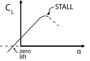
This surprisingly simple expression is a major finding of the thin air foil theory in the description of the lift force as determined by the foil angle of attack. This is based on a two-dimensional steady flow (or infinitely wide foil) with very little camber with viscous effects ignored. Some additional features and effects will be added to this equation later. Figure 6.7, shows the lift coefficient versus angle of attack. At large angles of attack the results of eqn. (6.21) are not valid. This is because the angle is so large that flow over the leading edge cannot negotiate the needed turn to stay “attached” to the foil surface. Rather the flow “separates” from following the surface contour. This results in a recirculating flow region between the streamlines of flow and the body surface. This can be seen in Figure 4.5 illustrating flow going over the leading edge of a thin airfoil at a fairly large angle of attack.

The primary limitation on the application of thin airfoil theory is the assumption of inviscid flow (which is actually has been shown to be a fairly valid approximation since all of the friction induced vorticity is accounted for with the vortex sheet). Also, the foil must be thin (maximum thickness on the order of ten percent of the chord length). This is not necessarily that restrictive since even airfoils with thicknesses of over 10% of the chord follow thin airfoil theory fairly well. With some modifications to the basic lift result of Equation \ref{6.19} thickness effects, relatively large camber and three-dimensional effects can be accounted for, as given below. A generic plot of the lift coefficient, \(C_L\), versus angle of attack, a, is given in Figure 6.7, as well as results for a specific airfoil, the NACA 0012 compared with Equation \ref{6.21}. Very good agreement between data and theory are shown up to an angle of attack of about 16^o.

Circulatory Lift: A Simple Method to Define Lift for an Airfoil

In this section we present an alternative approach to determining the lift for an airfoil. Consider a two-dimensional steady flow (a very wide airfoil) with the goal of determining the lift force versus angle of attack. There are much more rigorous methods to do this, involving complex variable representation of the flow. However, this simple treatment is rather straight forward and yields the same result in a more intuitive manner. The goal here is to illustrate from a flow physics point of view how the circulation is related to the lift force, and without circulation the lift force vanishes.

The no-slip boundary condition at the surface of the airfoil generates vorticity along the surface of the wing. For a perfectly symmetric wing that is oriented along the incoming flow direction the streamlines above and below the foil are identical. One can also imagine that the vorticity distribution on the top of the wing generated by surface friction is identical in magnitude but opposite in sign on the bottom of the wing (the rotation direction is opposite). Consequently, the sum total of vorticity around the wing becomes zero for this situation. However, tilting the wing at a given angle of attack relative to an in-coming flow creates an asymmetry of flow. See Figure 6.8 below. Notice in the figure that the flow leaves the trailing edge of the wing with a net downward flow direction either due to the camber or a tilting of the chord line relative to the freestream flow direction. In fact, in a vector sense the downward momentum of the flow has to have been generated by some downward force acting on the fluid. Selecting a rectangular control volume surrounding the wing and using this to integrate the velocity field along the surface of the control volume area as shown determines the magnitude of the circulation as:

\[\Gamma=\ \oint{V\bullet d s=}\iint_{A}{\omega\bullet d A}\]

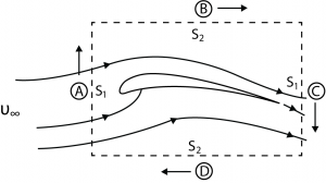
Where the line integral of the velocity is around the boundary of the area associated with the area of the vorticity integral. The contributions to the line integral for the different sides of the area are:

A: = \(0\) (there is no velocity component along this length (dot product of \(V\) and \(ds\) is zero)

B: ~\(U_\infty S_2\) (the boundary is far from the wing surface so the velocity is close to \(U_\infty\))

C: ~\(Ws1 S_1\) (\(W\) is the downward velocity component of the flow coming off of the trailing -edge which is assumed to be parallel with the top of the airfoil)

D: ~\(-U_\infty S_2\) (negative since the velocity is in the opposite direction as the integration)

By summing these components to obtain the total integration becomes \(\Gamma = WS_1\). This shows that the circulation is equal to the amount of downflow generated as the flow passes the airfoil. The lift force on the wing is equal and opposite to the force on the fluid. Using the momentum equation to determine the relationship between the force on the fluid and the change of momentum of the fluid results in (where forces are primed to represent force per span into the page):

\[F’ = ��’ = ��̇ �� = (\rho S_1 U_\infty)�� = \rho U_\infty) \Gamma\]

This illustrates that any object generating a downflow velocity in the control region will result in a net lift force on the object balancing the change of momentum of the fluid in the vertical direction. Also, this force is seen to be directly proportional to the circulation set up around the object. The assumption here is of irrotational flow outside of the viscous boundary layer so that there are no other sources of vorticity inside the selected control volume.

A slightly modified version of this can be used to determine the lift coefficient as well. Imaging a circle drawn around the wing with its center at the center of the wing (radius of , where \(c\) is the chord length). With this radius the circle will pass through the leading edge and trailing edge. Performing the line integral of the velocity component aligned with the circumference of the circle (dotting the velocity with \(ds\)) around the entire circle and using the notation of “W” being the net velocity component downward around the circle results in:

\[\Gamma\oint{V\bullet d s=W\oint d s=W2\pi\left(\frac{c}{2}\right)=\pi cW}\]

The lift force per span is then

\[L^\prime=\rho sU_\infty(\pi cW)\]

The lift coefficient is the lift force per area (sc) divided by

The ratio of the downwash velocity to the freestream velocity can be estimated as sin a, with a being the angle of attack, which results in:

\[C_L = 2 \pi \sin \alpha\]

This is the same result obtained using the more rigorous thin airfoil theory which helps to provide some physical insight into the role of the airfoil in defecting flow to obtain a net lift force.

Other Considerations of Forces

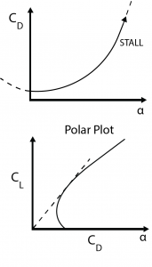
As stated previously the lift force is one component of the total force, the other component being the drag force. The drag force, \(D\), can be expressed as a drag coefficient, , similar to the lift coefficient. Although the drag force varies with angle of attack, unlike the lift coefficient it is fairly constant for a wide range of angle of attack prior to separation as shown in the figure below, except at fairly large angle of attack approaching the stall limit. Near zero angle of attack for a symmetric airfoil this drag is dominated by frictional forces acting on the foil surface. Another representation for the lift and drag coefficient is a “polar” plot which shows how the lift coefficient changes with drag coefficient. An example is shown below where the tangent line provides the minimum lift to drag ratio.

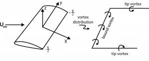
As stated previously there may be effects on the lift and drag forces caused by finite span (three-dimensional) wings, thickness and camber that would need to be taken into account. Finite span wings are obviously a reality and the fact that the ends of the wing (wing tips) causes flow conditions in the tip region to change. Specifically, the high pressure that exists below the wing meets with the low pressure on the top of the wing creating the tendency for a tip vortex to form. The resultant flow is a swirling flow directed from the bottom to the top of the wing. This appears as a vortex flow whose axis of rotation aligns closely with the direction of the freestream velocity. As the wing moves through the fluid the vortex axis extends out behind the wing. In fact, this phenomena for airplanes flying at sufficiently high altitudes the vortex motion results in a very low pressure at the center of the tip vorticities. The drop in pressure can cause water vapor to condense resulting in vapor trails or contrails forming at the wing tips that can be seen on the ground as a plan passes overhead. This phenomenon does have some negative effects on the performance of the wing.

The span of a wing determines how significant the tip vortex is on overall forces. A wing can be designated based on its span to chord length ratio (or aspect ratio). The term wing span of an aircraft typically includes the distance from tip to tip of the wings on an airplane – or twice the span of each wing. For a given wing however, the span is from the root to the tip. Denoting span by “s” and chord by “c” the aspect ratio is then . The swirling flow that results near the tip has flow coming up from the bottom, around the tip and then down onto the top of the wing. This downflow will have a tendency to divert the oncoming flow over the wing downward such that there is effectively a smaller angle of attack as seen by the wing. The axis of the vortex near the tip is characterized by the vortex line shown in the figure below extending backwards from the tip. In addition to this a “bound” vortex occurs around the wing due to the previously discussed vorticity distribution, with an axis of rotation along the wing span.

An induced angle of attack is defined as the amount of change (reduction) of the angle of attack as caused by the top vortex:

\[\alpha_{eff} = \alpha - \alpha_{induced}\]

The strength of \(\alpha_{induced}\) is given in terms of the downflow velocity induced by the tip vortex as:

\[\alpha_{induced}=tan^{−1}\frac{W}{U_\infty}{~}\frac{W}{U_\infty}\]

Where the later approximation is due to small angles since \(W << U_\infty\). Shown here without derivation, the total circulation accounting for the downwash effect written in terms of \(\alpha_{eff}\) is:

\[\Gamma\pi cU_\infty\alpha_{eff}\]

Using this expression for the circulation to determine the lift after some manipulation the lift coefficient becomes:

\[C_L=\frac{2\pi\alpha}{1+\frac{2c}{s}}\]

In the limit of large aspect ratio, or becoming small, the lift coefficient reverts to that for an infinite span wing as expected. Also, there is an induced drag that is set up from the downflow which can be determined in terms of the lift coefficient to be:

\[C_D=C_{Do}+C_{D,\ induced}\]

where \(CD,o\) is the drag coefficient for an infinite wing.

There is also an effect caused by asymmetry in the foil geometry such as camber. In this case the camber adds to the asymmetry of the foil as shown in Figure 6.6. The maximum camber along the chord line is designated as “h” and the maximum thickness as “t”.

For cambered foils the lift becomes:

\[\Gamma=\pi sU_\infty\left(1+0.77\frac{t}{c}\right)\sin{\left(\alpha+\beta\right)}\]

\[\beta tan^{−1}\left(\frac{2h}{c}\right)\]

As the camber increases, by increasing , and therefor increasing \(\beta\), the circulation increases. Using this to define the lift coefficient we have the following relationship that accounts for both finite span wings and camber asymmetry:

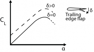
The effect of an artificially imposed camber is shown in the figure below by using a flap at the rear of the foil. There can be a significant increase in lift when deploying a flap, and this provides a means to increase lift as needed.

Airfoil shapes are often designated by different “codes” or “designations”. An early form of this was developed by NACA (National Advisory Committee for Aeronautics, a precursor to NASA). Several such designations have been developed such as the 4, 5 and 6 digit numerical designations as are shown below based on camber, location of maximum camber and thickness. More elaborate designations have been developed over the years.