3.1: Built-In Functions

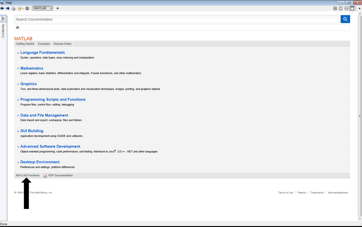
As with most parts of Matlab, the Help window is useful in describing the functions that are in Matlab, Simulink, and any toolbox add-ons that you may have. To access the entire list of functions, grouped in various ways, click on the Help button, the one shaped like a question mark at the top of the main Matlab window, or simply use the F1 button. Once on the Help window, you can click on “MATLAB Functions” at the bottom.

In discovering what a function does, we suggest to simply try it. Let’s start with the matrix A = [1 2 49 4;25 36 3 81] and look at the output from several functions. First type in
>> A = [1 2 49 4;25 36 3 81]

• sqrt(A)

The output:

>> sqrt(A)
ans =
1.0000 1.4142 7.0000 2.0000
5.0000 6.0000 1.7321 9.0000

is (hopefully) what you might expect. It finds the square root of each of the entries. If you know a little more linear algebra and was expecting the “principal” square root, or a matrix B so that B * B = A, this is created using B = sqrtm(A).

• sin(A), sind(A)

The function sin(A) finds the sine of every entry in A, assuming the entries of A are in radians:

>> sin(A)

ans =
0.8415 0.9093 -0.9538 -0.7568
-0.1324 -0.9918 0.1411 -0.6299

and the function sind(A) does the same, but assumes the entries of A are in degrees:

>> sind(A)

ans =
0.0175 0.0349 0.7547 0.0698
0.4226 0.5878 0.0523 0.9877

The other trigonometric functions are similarly named.

• exp(A), log(A), log10(A)

These three functions are base e exponentiation, the natural log and the logarithm base 10. They act entry-wise:

>> exp(A)

ans =
1.0e+035 *
0.0000 0.0000 0.0000 0.0000
0.0000 0.0000 0.0000 1.5061

>> log(A)

ans =

0 0.6931 3.8918 1.3863
3.2189 3.5835 1.0986 4.3944

>> log10(A)

ans =

0 0.3010 1.6902 0.6021
1.3979 1.5563 0.4771 1.9085

We do see something curious here for the function exp(A). It looks like all of the entries are zero until a closer look shows the leading term “1.0e+035 *”. This means that every entry in the answer is multiplied by this factor 1035 (a rather large number). The fact that the other entries look like zero is that there aren’t enough decimal places to store each answer.

• mean(A), median(A), std(A)

These are some of the basic statistical functions. The output for these are the mean, median, and standard deviation of the columns of A.

>> mean(A)

ans =
13.0000 19.0000 26.0000 42.5000

>> std(A)

ans =
16.9706 24.0416 32.5269 54.4472

>> median(A)

ans =
13.0000 19.0000 26.0000 42.5000

• sort(A), sortrows(A)

The command sort rearranges the data in the columns of A in increasing order. The command sortrows sorts the rows of A in increasing order (deter-
mined by the first column).

>> sort(A)

ans =
1 2 3 4
25 36 49 81

>> sortrows(A)

ans =
1 2 49 4
25 36 3 81

However, both of these functions can take other arguments. For example, the sort function can also be used to sort the columns, or can sort using either ‘descend’ or ‘ascend’. The sortrows function can also be used to sort according to other columns. See the Help files for more details.

• flipud(A), fliplr(A)

These two functions are abbreviations of “flip up-and-down” and “flip left-to-right”. That’s exactly what they do:

>> flipud(A)

ans =
25 36 3 81
1 2 49 4

>> fliplr(A)

ans =
4 49 2 1
81 3 36 25

• find

The function find is used to located the position of values in a matrix.

>> find(A==1)

ans =
1
A couple of comments about this example. First, there is a double equals sign in A==1. There will be more about this in a future chapter (on relational operators), but you can read this as a question “does A equal 1?.” The entire line find(A==1) indicates the location where the (element of) A does in fact equal 1 (namely the first entry). Another example:

>> find(a>5)

ans =
2
4
5
8
Here we must again remember to read down the columns of A to get to the 2nd, 4th, 5th and 8th entries. We can tweak this last example to get the exact rows and columns containing entries greater than 5:

>> [r,c]=find(A>5);[r,c]

ans =
2 1
2 2
1 3
2 4
Here we have given the find function two outputs to write to, the variables r and c, which are displayed together for easier reading using [r,c]. The output indicates that the entries of A that are greater than 5 can be found in the 2nd row & 1st column, 2nd row & 2nd column, 1st row & 3rd column, and 2nd row & 4th column.

In the next example, we investigate the function meshgrid. The meshgrid function is used to transform vectors x and y into arrays X and Y of sizes appropriate for computation and plotting.

Example 3.1.1: Using meshgrid

Suppose we wanted to compute the area of a triangle for all possible combinations of the base, ranging from 7 to 10 units, and the height, ranging from 2 to 6 units. Here’s the set up (output suppressed):

>> Base = 7:10;

>> Height = 2:6;

Now, we can’t just multiply these two matrices together, nor can we “dot multiply” them either, since the dimensions of Base, 1 × 4, and Height, 1 × 5, do not line up properly in either case. Instead we resize using meshgrid:

>> [NewBase,NewHeight] = meshgrid(Base,Height)

This creates two matrices, NewBase and NewHeight, which are both 5×4. We did not suppress the output, so one can see that these are:

NewBase =
7 8 9 10
7 8 9 10
7 8 9 10
7 8 9 10
7 8 9 10

and

NewHeight =
2 2 2 2
3 3 3 3
4 4 4 4
5 5 5 5
6 6 6 6
We can now “dot multiply” them together:

>> Area= (NewBase.*NewHeight)/2

Area =
7.0000 8.0000 9.0000 10.0000
10.5000 12.0000 13.5000 15.0000
14.0000 16.0000 18.0000 20.0000
17.5000 20.0000 22.5000 25.0000
21.0000 24.0000 27.0000 30.0000