6.1: Input Commands

In order to run either script M-files or function M-files, the user needs to provide data, either numerical or text (“strings”). The first command we consider is simply called input.

Example 6.1.1: Using the input command

Here is a simple section of code to collect a person’s first name and their age.

>> FirstName = input('Enter your first name : ','s');
>> Age = input('Enter your age : ');

Once executed, the user enters values for each, say

Enter your first name : Bob
Enter your age : 25

In this example, the 's' in the first input indicates that the program expects text input and the second input (without the 's') indicates that the program expects numeric input. When executed, the lines collect input one at a time. Note the text Waiting for input on the bottom left of the Matlab window while the user enters the name, Bob, and age, 25. Due to the semicolons, there is no output to the screen, but the values have been stored in the variables FirstName and Age (see the Workspace window to confirm).

So how do we display this information? There are several ways to output this information. Here we consider the two commands disp (for “display”) and fprintf (“formated print to file”). The help files are useful so look them up!

We can present this information as follows.

Example 6.1.2: Using the disp command

Using the data from the last example:

>> disp('Your first name is ')
>> disp(FirstName)
>> disp('Your age is ')
>> disp(Age)

which has the output:

Your first name is
Bob
Your age is
25

This example is ok, but it would be nicer if the data was in one line. That’s where the command fprintf comes in. Even though it is a formatted print “to file” you can have the output sent to the Command Window instead.

Example 6.1.3: Using the command fprintf

>> fprintf('%s is %.0f years old.\n ',FirstName,Age)

produces

Bob is 25 years old.

Certainly, there is more involved in the function fprintf in order to produce the output we want. Let’s look at the individual pieces of this example.

• The % signs are NOT for comments this time (note: they aren’t green), they are now used as place holders for the data.
• The %s indicates that a string is expected as input.
• The %.0f indicates that we expect a numeric input, want zero decimal points and the value should be in Fixed-point format. For more information on specific formats and “conversion characters” (which is what f and s are here), look at the fprintf command in the help files.
• The \n is an “escape character” that creates a New Line.
• The data FirstName and Age are listed after this, separated by commas.
• When the command is run, Matlab places the first data value, FirstName (i.e. Bob), in the %s position and the second data value, Age (i.e. 25), in the %.0f position. Got it?

Just for completeness, we can also force the disp command to act like fprintf as follows:

Example 6.1.4: disp using concatenated strings

>> disp([FirstName,' is ', num2str(Age),' years old.'])

produces

Bob is 25 years old.

Basically, we are displaying a string array made up of several strings through concatenation. We also see the command num2str which does exactly what it says, it converts a number into a string. This is necessary since numeric data and strings don’t play well together in Matlab. In order to create a string array, all of the parts must be strings. If we tried to run this without the num2str command, we would get

>> disp([FirstName,' is ', Age,' years old.'])

with output

Bob is years old.

where the square indicates that the ASCII code for the value 25 is unprintable (look it up or don’t worry about it - just remember the num2str).

Let’s look at how to read and write larger data files next.

Example 6.1.5

Create the following table of years and monthly world steel production (in thousand metric tons) in an Excel file and save the file as WorldSteelProduction.xls (or .xlsx). Make sure to save this file in the directory listed at the top of the Matlab window, the Currect Directory.

2005	2006	2007	2008	2009	2010
91377	95037	107789	112870	86476	113375
84980	91183	101465	107465	86610	107119
93198	102183	112988	119934	92144	122196
93381	101604	110241	117023	89644	120497
95290	105501	112933	121062	96177	124567
92095	104636	112159	118851	100661	118346
90205	104350	110377	116770	104701	114365
91536	102630	109024	112726	108351	113141
93144	103676	111956	107723	110773	112340
98534	106913	114703	99202	114765	117377
94340	104817	109936	86513	108596	114637
95368	105306	111506	81704	107792	116157

We will now read in this data using xlsread, plot it, and access data from it using the mouse and the graphical input command ginput (“gee-input”).

>> Steel = xlsread('WorldSteelProduction.xls');

Next, we plot the data

>> plot(1:12,Steel(2:end,:))
>> legend('2005','2006','2007','2008','2009','2010', ...'Location','best')

The initial problem is to find the first time in 2009 that steel production is at 100,000 thousand metric tons. We use the ginput command for the user to collect this data.

>> disp('Select the 2009 time when production is 100,000.');
>> [t,l] = ginput(1) % mouse click

If the user hovers the cursor over the resulting plot, we see cross-hairs appear:

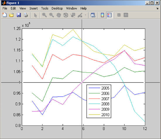
A left-click creates the output to appear in the Command Window:

t =
5.8756
l =
9.9934e+004

Note that the level is listed in engineering format. If we want to finish this example with a formatted output, we could use the following:

>> fprintf('Level %6.1f occurs %3.1f months into 2009.\n',l,t)

Level 99934.2 occurs 5.9 months into 2009.

which is in mid-June 2009. Note that the accuracy of the level and time are dependent on the user’s mouse click so the output may not look exactly the same.
(Data from http://www.worldsteel.org/)

Key Idea 2

fprintf with matrices

If there are not enough place holders, fprintf will cycle through the values in the given data matrix, USING COLUMN PRECEDENCE, until all of the values are exhausted.

Example 6.1.6

Here we use fprintf and Key Idea 2 to display a matrix of values. Find the sine, cosine and tangent of theta from 0 to 2π by steps of π/10.

>> theta=[0:pi/10:2*pi];
>> values=[theta;sin(theta);cos(theta);tan(theta)];

To display these, we can use a simple fprintf.

>> disp('Theta Sine Cosine Tangent ');
>> fprintf('%5.2f %6.2f %7.2f %9.2f\ n ',values)

gives output:

Theta Sine Cosine Tangent
0.00 0.00 1.00 0.00
0.31 0.31 0.95 0.32
0.63 0.59 0.81 0.73
0.94 0.81 0.59 1.38
1.26 0.95 0.31 3.08
1.57 1.00 0.00 16331239353195370.00
1.88 0.95 -0.31 -3.08
2.20 0.81 -0.59 -1.38
2.51 0.59 -0.81 -0.73
2.83 0.31 -0.95 -0.32
3.14 0.00 -1.00 -0.00
3.46 -0.31 -0.95 0.32
3.77 -0.59 -0.81 0.73
4.08 -0.81 -0.59 1.38
4.40 -0.95 -0.31 3.08
4.71 -1.00 -0.00 5443746451065123.00
5.03 -0.95 0.31 -3.08
5.34 -0.81 0.59 -1.38
5.65 -0.59 0.81 -0.73
5.97 -0.31 0.95 -0.32
6.28 -0.00 1.00 -0.00

In this example, the reason for the large values in the last column are because the tangent function tends to infinity as the angle tends to π/2 (and 1.5708 is close to π/2). Actually, the value tan(π/2) returns 1.6331e+016. Why isn’t “infinity” the returned value? Well, it has to do with how values are stored in Matlab (using double-precision). The value 1.6331e+016 is actually the reciprocal of the value eps = 10∧(-52). If you want to know more, head to the help files (or Google, of course).