16.1: Curve Fitting

Data sets are by definition a discrete set of points. We can plot them, but we often want to view trends, interpolate new points and (carefully!) extrapolate for prediction purposes. Linear regression is a powerful tool, although sometimes the data would be better fit by another curve. Here we show how to do linear and quadratic regression.

Example 16.1.1

Consider the following data set from example 15.1.1 in the previous chapter.

\[F:=\begin{pmatrix}
2\\
4\\
6\\
8\\
10\\
12\\
14\\
16\\
18\\
20
\end{pmatrix}.kN\nonumber\]

\[δ:=\begin{pmatrix}
0.82\\
1.47\\
2.05\\
3.37\\
3.75\\
4.17\\
5.25\\
5.44\\
6.62\\
7.97
\end{pmatrix}.mm\nonumber\]

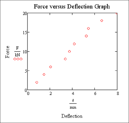
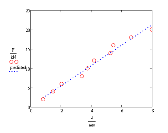
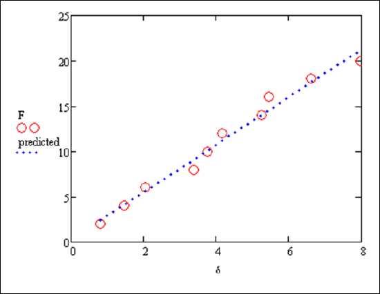
Let’s find the least squares line. We consider two methods to do this.

Method 1

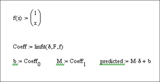
Method 2

This method uses the command linfit. It is a bit awkward here, but will be useful when we do higher order regression. We do have to first remove the units from our variables (a limitation of linfit)

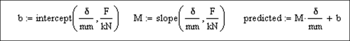
Now put them together on the same plot:

Example 16.1.2

Consider the following data set:

\[Time:=\begin{pmatrix}
0\\
1\\
2\\
3\\
4\\
5\\
6
\end{pmatrix}\nonumber\]

\[Distance2:=\begin{pmatrix}
5\\
19.8\\
76.8\\
153.3\\
256.2\\
394.5\\
559.2
\end{pmatrix}\nonumber\]

Plotted:

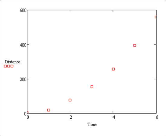
The plot of the data suggests a quadratic fit, i.e. a curve y = a + bx + cx².

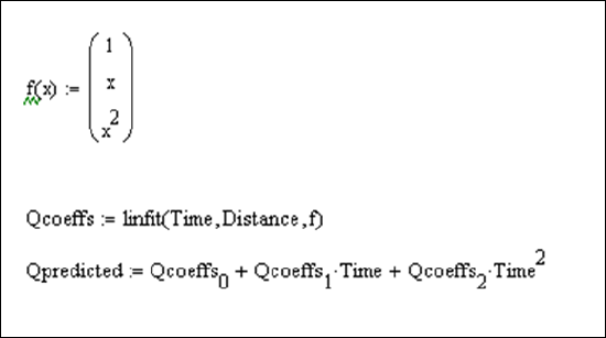
How do we find this quadratic curve?
Here’s how we implement this in Mathcad:

Now plot them together:

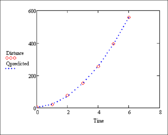
We can compute the R-squared value to see the correlation between Distance and Qpredicted.

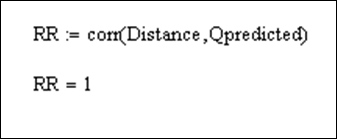
'RR=1' means a great fit.