2.3: The backpropagation algorithm
- Page ID
- 3747
The backpropagation equations provide us with a way of computing the gradient of the cost function. Let's explicitly write this out in the form of an algorithm:
- Input \(x\): Set the corresponding activation \(a^1\) for the input layer.
- Feedforward: For each \(l=2,3,…,L\) compute \(z^l = w^la^{l-1}+b^l \) and \(a^l = σ(z^l)\).
- Output error \(δ^L\): Compute the vector \(δ^L= ∇_a C⊙σ′(z^L)\).
- Backpropagate the error: For each \(l=L−1,L−2,…,2\) compute \(δ^l =((w^{l+1})^T δ^{l+1})⊙σ′(z^l)\).
- Output: The gradient of the cost function is given by \(\frac{∂C}{∂w^l_{jk}} =a^{l−1}_k δ^l_j\) and \(\frac{∂C}{∂b^l_j} = δ^l_j\).
Examining the algorithm you can see why it's called backpropagation. We compute the error vectors \(δ^l\) backward, starting from the final layer. It may seem peculiar that we're going through the network backward. But if you think about the proof of backpropagation, the backward movement is a consequence of the fact that the cost is a function of outputs from the network. To understand how the cost varies with earlier weights and biases we need to repeatedly apply the chain rule, working backward through the layers to obtain usable expressions.
Exercises
- Backpropagation with a single modified neuronSuppose we modify a single neuron in a feedforward network so that the output from the neuron is given by \(f(\sum_jw_jx_j + b)\), where \(f\) is some function other than the sigmoid. How should we modify the backpropagation algorithm in this case?
- Backpropagation with linear neurons Suppose we replace the usual non-linear \(σ\) function with \(σ(z)=z\) throughout the network. Rewrite the backpropagation algorithm for this case.
As I've described it above, the backpropagation algorithm computes the gradient of the cost function for a single training example, \(C=C_x\). In practice, it's common to combine backpropagation with a learning algorithm such as stochastic gradient descent, in which we compute the gradient for many training examples. In particular, given a mini-batch of mm training examples, the following algorithm applies a gradient descent learning step based on that mini-batch:
- Input a set of training examples
- For each training example \(x\): Set the corresponding input activation \(a^{x,1}\) and perform the following steps:
- Feedforward: For each \(l=2,3,…,L\) compute \(z^{x,l} = w^l a^{x,l−1} + b^l\) and \(a^{x,l} = σ(z^{x,l})\).
- Output error \(δ^{x,L}\): Compute the vector \(δ^{x,L}\) = ∇_aC_x ⊙ σ′(z^{x,L})\).
- Backpropagate the error: For each \(l=L−1,L−2,…,2\) compute \(δ^{x,l} = ((w^{l+1})^T δ^{x,l+1}) ⊙ σ′(z^{x,l})\).
- Gradient descent: For each \(l=L,L−1,…,2\) update the weights according to the rule \(w^l→ w^l−\frac{η}{m}\sum_x δ^{x,l} (a^{x,l−1})^T \), and the biases according to the rule \(b^l→b^l −\frac{η}{m}\sum_x δ^{x,l}\).
Of course, to implement stochastic gradient descent in practice you also need an outer loop generating mini-batches of training examples, and an outer loop stepping through multiple epochs of training. I've omitted those for simplicity.
The code for backpropagation
Having understood backpropagation in the abstract, we can now understand the code used in the last chapter to implement backpropagation. Recall from that chapter that the code was contained in the update_mini_batch and backprop methods of the Network class. The code for these methods is a direct translation of the algorithm described above. In particular, the update_mini_batch method updates the Network's weights and biases by computing the gradient for the current mini_batch of training examples:
class Network(object):
...
    def update_mini_batch(self, mini_batch, eta):
        """Update the network's weights and biases by applying
        gradient descent using backpropagation to a single mini batch.
        The "mini_batch" is a list of tuples "(x, y)", and "eta"
        is the learning rate."""
        nabla_b = [np.zeros(b.shape) for b in self.biases]
        nabla_w = [np.zeros(w.shape) for w in self.weights]
        for x, y in mini_batch:
            delta_nabla_b, delta_nabla_w = self.backprop(x, y)
            nabla_b = [nb+dnb for nb, dnb in zip(nabla_b, delta_nabla_b)]
            nabla_w = [nw+dnw for nw, dnw in zip(nabla_w, delta_nabla_w)]
        self.weights = [w-(eta/len(mini_batch))*nw
                        for w, nw in zip(self.weights, nabla_w)]
        self.biases = [b-(eta/len(mini_batch))*nb
                       for b, nb in zip(self.biases, nabla_b)]
Most of the work is done by the line delta_nabla_b, delta_nabla_w = self.backprop(x, y) which uses the backprop method to figure out the partial derivatives \(∂C_x/∂b^l_j\) and \(∂C_x/∂w^l_{jk}\). The backprop method follows the algorithm in the last section closely. There is one small change - we use a slightly different approach to indexing the layers. This change is made to take advantage of a feature of Python, namely the use of negative list indices to count backward from the end of a list, so, e.g., l[-3] is the third last entry in a list l. The code for backprop is below, together with a few helper functions, which are used to compute the \(σ\) function, the derivative \(σ′\), and the derivative of the cost function. With these inclusions you should be able to understand the code in a self-contained way. If something's tripping you up, you may find it helpful to consult the original description (and complete listing) of the code.
class Network(object):
...
   def backprop(self, x, y):
        """Return a tuple "(nabla_b, nabla_w)" representing the
        gradient for the cost function C_x.  "nabla_b" and
        "nabla_w" are layer-by-layer lists of numpy arrays, similar
        to "self.biases" and "self.weights"."""
        nabla_b = [np.zeros(b.shape) for b in self.biases]
        nabla_w = [np.zeros(w.shape) for w in self.weights]
        # feedforward
        activation = x
        activations = [x] # list to store all the activations, layer by layer
        zs = [] # list to store all the z vectors, layer by layer
        for b, w in zip(self.biases, self.weights):
            z = np.dot(w, activation)+b
            zs.append(z)
            activation = sigmoid(z)
            activations.append(activation)
        # backward pass
        delta = self.cost_derivative(activations[-1], y) * \
            sigmoid_prime(zs[-1])
        nabla_b[-1] = delta
        nabla_w[-1] = np.dot(delta, activations[-2].transpose())
        # Note that the variable l in the loop below is used a little
        # differently to the notation in Chapter 2 of the book.  Here,
        # l = 1 means the last layer of neurons, l = 2 is the
        # second-last layer, and so on.  It's a renumbering of the
        # scheme in the book, used here to take advantage of the fact
        # that Python can use negative indices in lists.
        for l in xrange(2, self.num_layers):
            z = zs[-l]
            sp = sigmoid_prime(z)
            delta = np.dot(self.weights[-l+1].transpose(), delta) * sp
            nabla_b[-l] = delta
            nabla_w[-l] = np.dot(delta, activations[-l-1].transpose())
        return (nabla_b, nabla_w)

...

    def cost_derivative(self, output_activations, y):
        """Return the vector of partial derivatives \partial C_x /
        \partial a for the output activations."""
        return (output_activations-y)

def sigmoid(z):
    """The sigmoid function."""
    return 1.0/(1.0+np.exp(-z))

def sigmoid_prime(z):
    """Derivative of the sigmoid function."""
    return sigmoid(z)*(1-sigmoid(z))
Problem
- Fully matrix-based approach to backpropagation over a mini-batch Our implementation of stochastic gradient descent loops over training examples in a mini-batch. It's possible to modify the backpropagation algorithm so that it computes the gradients for all training examples in a mini-batch simultaneously. The idea is that instead of beginning with a single input vector, x, we can begin with a matrix \(X=[x_1x_2…x_m]\) whose columns are the vectors in the mini-batch. We forward-propagate by multiplying by the weight matrices, adding a suitable matrix for the bias terms, and applying the sigmoid function everywhere. We backpropagate along similar lines. Explicitly write out pseudocode for this approach to the backpropagation algorithm. Modify network.py so that it uses this fully matrix-based approach. The advantage of this approach is that it takes full advantage of modern libraries for linear algebra. As a result it can be quite a bit faster than looping over the mini-batch. (On my laptop, for example, the speedup is about a factor of two when run on MNIST classification problems like those we considered in the last chapter.) In practice, all serious libraries for backpropagation use this fully matrix-based approach or some variant.
In what sense is backpropagation a fast algorithm?
In what sense is backpropagation a fast algorithm? To answer this question, let's consider another approach to computing the gradient. Imagine it's the early days of neural networks research. Maybe it's the 1950s or 1960s, and you're the first person in the world to think of using gradient descent to learn! But to make the idea work you need a way of computing the gradient of the cost function. You think back to your knowledge of calculus, and decide to see if you can use the chain rule to compute the gradient. But after playing around a bit, the algebra looks complicated, and you get discouraged. So you try to find another approach. You decide to regard the cost as a function of the weights \(C=C(w)\) alone (we'll get back to the biases in a moment). You number the weights \(w_1,w_2,…\), and want to compute \(∂C/∂w_j\) for some particular weight \(w_j\). An obvious way of doing that is to use the approximation
\[ \frac{∂C}{∂w_j} ≈ \frac{C(w+ϵe_j) − C(w)}{ϵ},\label{46}\tag{46} \]
where \(ϵ>0\) is a small positive number, and \(e_j\) is the unit vector in the \(j^{th}\) direction. In other words, we can estimate \(∂C/∂w_j\) by computing the cost \(C\) for two slightly different values of \(w_j\), and then applying Equation \(\ref{46}\). The same idea will let us compute the partial derivatives \(∂C/∂b\) with respect to the biases.
This approach looks very promising. It's simple conceptually, and extremely easy to implement, using just a few lines of code. Certainly, it looks much more promising than the idea of using the chain rule to compute the gradient!
Unfortunately, while this approach appears promising, when you implement the code it turns out to be extremely slow. To understand why, imagine we have a million weights in our network. Then for each distinct weight \(w_j\) we need to compute \(C(w+ϵe_j)\) in order to compute \(∂C/∂w_j\). That means that to compute the gradient we need to compute the cost function a million different times, requiring a million forward passes through the network (per training example). We need to compute \(C(w)\) as well, so that's a total of a million and one passes through the network.
What's clever about backpropagation is that it enables us to simultaneously compute all the partial derivatives \(∂C/∂w_j\) using just one forward pass through the network, followed by one backward pass through the network. Roughly speaking, the computational cost of the backward pass is about the same as the forward pass*
*This should be plausible, but it requires some analysis to make a careful statement. It's plausible because the dominant computational cost in the forward pass is multiplying by the weight matrices, while in the backward pass it's multiplying by the transposes of the weight matrices. These operations obviously have similar computational cost.
And so the total cost of backpropagation is roughly the same as making just two forward passes through the network. Compare that to the million and one forward passes we needed for the approach based on \(\ref{46}\)! And so even though backpropagation appears superficially more complex than the approach based on \(\ref{46}\), it's actually much, much faster.
This speedup was first fully appreciated in 1986, and it greatly expanded the range of problems that neural networks could solve. That, in turn, caused a rush of people using neural networks. Of course, backpropagation is not a panacea. Even in the late 1980s people ran up against limits, especially when attempting to use backpropagation to train deep neural networks, i.e., networks with many hidden layers. Later in the book we'll see how modern computers and some clever new ideas now make it possible to use backpropagation to train such deep neural networks.
Backpropagation: the big picture
As I've explained it, backpropagation presents two mysteries. First, what's the algorithm really doing? We've developed a picture of the error being backpropagated from the output. But can we go any deeper, and build up more intuition about what is going on when we do all these matrix and vector multiplications? The second mystery is how someone could ever have discovered backpropagation in the first place? It's one thing to follow the steps in an algorithm, or even to follow the proof that the algorithm works. But that doesn't mean you understand the problem so well that you could have discovered the algorithm in the first place. Is there a plausible line of reasoning that could have led you to discover the backpropagation algorithm? In this section I'll address both these mysteries.
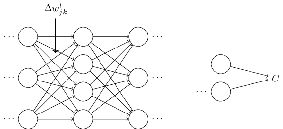
To improve our intuition about what the algorithm is doing, let's imagine that we've made a small change \(Δw^l_{jk}\) to some weight in the network, \(w^l_{jk}\):
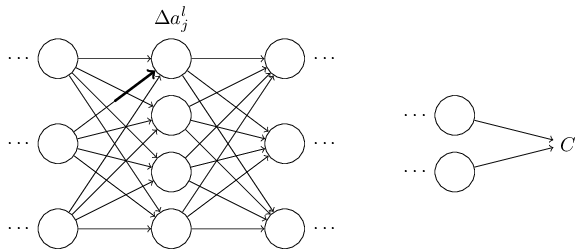
That change in weight will cause a change in the output activation from the corresponding neuron:
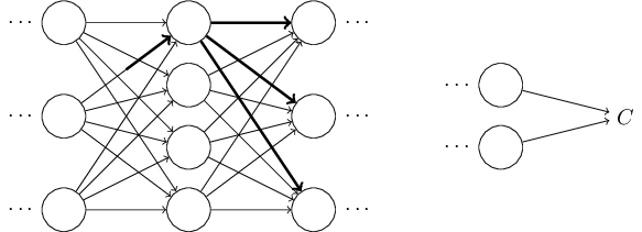
That, in turn, will cause a change in all the activations in the next layer:
Those changes will in turn cause changes in the next layer, and then the next, and so on all the way through to causing a change in the final layer, and then in the cost function:
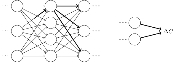
The change \(ΔC\) in the cost is related to the change \(Δw^l_{jk}\) in the weight by the equation
\[ ΔC ≈ \frac{∂C}{∂w^l_jk}Δw^l_{jk}\label{47} \tag{47}\]
This suggests that a possible approach to computing \(\frac{∂C}{∂w^l_{jk}}\) is to carefully track how a small change in \(w^l_{jk}\) propagates to cause a small change in \(C\). If we can do that, being careful to express everything along the way in terms of easily computable quantities, then we should be able to compute \(∂C/∂w^l_{jk}\).
Let's try to carry this out. The change \(Δw^l_{jk}\) causes a small change \(Δa^l_j\) in the activation of the \(j^{th}\) neuron in the \(l^{th}\) layer. This change is given by
\[ Δa^l_j ≈ \frac{∂a^l_j}{∂w^l_{jk}} Δw^l_{jk}\label{48} \tag{48}\]
The change in activation \(Δa^l_j\) will cause changes in all the activations in the next layer, i.e., the \((l+1)^{th}\). We'll concentrate on the way just a single one of those activations is affected, say \(a^{l+1}_q\),
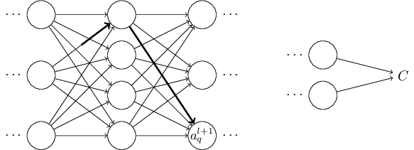
In fact, it'll cause the following change:
\[ Δa^{l+1}_q ≈ \frac{∂a^{l+1}_q}{∂a^l_j}\label{49}\tag{49} \]
Substituting in the expression from Equation \ref{48} we get:
\[ Δa^{l+1}_q ≈ \frac{∂a^{l+1}_q}{∂a^l_j} \frac{∂a^l_j}{∂w^l_{jk}}Δw^l_{jk}\label{50}\tag{50} \]
Of course, the change \(Δa^{l+1}_q\) will, in turn, cause changes in the activations in the next layer. In fact, we can imagine a path all the way through the network from \(w^l_{jk}\) to \(C\), with each change in activation causing a change in the next activation, and, finally, a change in the cost at the output. If the path goes through activations \(a^l_j,a^{l+1}_q,…,a^{L−1}_n,a^L_m\) then the resulting expression is
\[ ΔC≈\frac{∂C}{∂a^L_m}\frac{∂a^L_m}{∂a^{L−1}_n}\frac{∂a^{L−1}_n}{∂a^{L−2}_p}…\frac{∂a^{l+1}_q}{∂a^l_j}\frac{∂a^l_j}{∂w^l_{jk}}Δw^l_{jk},\label{51}\tag{51} \]
that is, we've picked up a \(∂a/∂a\) type term for each additional neuron we've passed through, as well as the \(∂C/∂a^L_m\) term at the end. This represents the change in \(C\) due to changes in the activations along this particular path through the network. Of course, there's many paths by which a change in \(w^l_{jk}\) can propagate to affect the cost, and we've been considering just a single path. To compute the total change in \(C\) it is plausible that we should sum over all the possible paths between the weight and the final cost, i.e.,
\[ ΔC≈\sum_{mnp…q}{\frac{∂C}{∂a^L_m}\frac{∂a^L_m}{∂a^{L−1}_n}\frac{∂a^{L−1}_n}{∂a^{L−2}_p}…\frac{∂a^{l+1}_q}{∂a^l_j}\frac{∂a^l_j}{∂w^l_{jk}}Δw^l_{jk}},\label{52}\tag{52} \]
where we've summed over all possible choices for the intermediate neurons along the path. Comparing with \(\ref{47}\) we see that
\[\frac{∂C}{∂w^l_{jk}} =\sum_{mnp…q}{\frac{∂C}{∂a^L_m}\frac{∂a^L_m}{∂a^{L−1}_n}\frac{∂a^{L−1}_n}{∂a^{L−2}_p}…\frac{∂a^{l+1}_q}{∂a^l_j}\frac{∂a^l_j}{∂w^l_{jk}}}.\label{53}\tag{53} \]
Now, Equation \(\ref{53}\) looks complicated. However, it has a nice intuitive interpretation. We're computing the rate of change of \(C\) with respect to a weight in the network. What the equation tells us is that every edge between two neurons in the network is associated with a rate factor which is just the partial derivative of one neuron's activation with respect to the other neuron's activation. The edge from the first weight to the first neuron has a rate factor \(∂a^l_j/∂w^l_{jk}\). The rate factor for a path is just the product of the rate factors along the path. And the total rate of change \(∂C/∂w^l_{jk}\) is just the sum of the rate factors of all paths from the initial weight to the final cost. This procedure is illustrated here, for a single path:
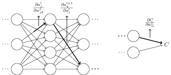
What I've been providing up to now is a heuristic argument, a way of thinking about what's going on when you perturb a weight in a network. Let me sketch out a line of thinking you could use to further develop this argument. First, you could derive explicit expressions for all the individual partial derivatives in Equation \(\ref{53}\). That's easy to do with a bit of calculus. Having done that, you could then try to figure out how to write all the sums over indices as matrix multiplications. This turns out to be tedious, and requires some persistence, but not extraordinary insight. After doing all this, and then simplifying as much as possible, what you discover is that you end up with exactly the backpropagation algorithm! And so you can think of the backpropagation algorithm as providing a way of computing the sum over the rate factor for all these paths. Or, to put it slightly differently, the backpropagation algorithm is a clever way of keeping track of small perturbations to the weights (and biases) as they propagate through the network, reach the output, and then affect the cost.
Now, I'm not going to work through all this here. It's messy and requires considerable care to work through all the details. If you're up for a challenge, you may enjoy attempting it. And even if not, I hope this line of thinking gives you some insight into what backpropagation is accomplishing.
What about the other mystery - how backpropagation could have been discovered in the first place? In fact, if you follow the approach I just sketched you will discover a proof of backpropagation. Unfortunately, the proof is quite a bit longer and more complicated than the one I described earlier in this chapter. So how was that short (but more mysterious) proof discovered? What you find when you write out all the details of the long proof is that, after the fact, there are several obvious simplifications staring you in the face. You make those simplifications, get a shorter proof, and write that out. And then several more obvious simplifications jump out at you. So you repeat again. The result after a few iterations is the proof we saw earlier* - short, but somewhat obscure, because all the signposts to its construction have been removed! I am, of course, asking you to trust me on this, but there really is no great mystery to the origin of the earlier proof. It's just a lot of hard work simplifying the proof I've sketched in this section.
*There is one clever step required. In Equation \(\ref{53}\) the intermediate variables are activations like \(a^{l+1}_q\). The clever idea is to switch to using weighted inputs, like \(z^{l+1}_q\), as the intermediate variables. If you don't have this idea, and instead continue using the activations \(a^{l+1}_q\), the proof you obtain turns out to be slightly more complex than the proof given earlier in the chapter.


