Engineering LibreTexts

5.2: Unstable gradients in more complex networks

  • Page ID
    3767
  • \( \newcommand{\vecs}[1]{\overset { \scriptstyle \rightharpoonup} {\mathbf{#1}} } \)

    \( \newcommand{\vecd}[1]{\overset{-\!-\!\rightharpoonup}{\vphantom{a}\smash {#1}}} \)

    \( \newcommand{\id}{\mathrm{id}}\) \( \newcommand{\Span}{\mathrm{span}}\)

    ( \newcommand{\kernel}{\mathrm{null}\,}\) \( \newcommand{\range}{\mathrm{range}\,}\)

    \( \newcommand{\RealPart}{\mathrm{Re}}\) \( \newcommand{\ImaginaryPart}{\mathrm{Im}}\)

    \( \newcommand{\Argument}{\mathrm{Arg}}\) \( \newcommand{\norm}[1]{\| #1 \|}\)

    \( \newcommand{\inner}[2]{\langle #1, #2 \rangle}\)

    \( \newcommand{\Span}{\mathrm{span}}\)

    \( \newcommand{\id}{\mathrm{id}}\)

    \( \newcommand{\Span}{\mathrm{span}}\)

    \( \newcommand{\kernel}{\mathrm{null}\,}\)

    \( \newcommand{\range}{\mathrm{range}\,}\)

    \( \newcommand{\RealPart}{\mathrm{Re}}\)

    \( \newcommand{\ImaginaryPart}{\mathrm{Im}}\)

    \( \newcommand{\Argument}{\mathrm{Arg}}\)

    \( \newcommand{\norm}[1]{\| #1 \|}\)

    \( \newcommand{\inner}[2]{\langle #1, #2 \rangle}\)

    \( \newcommand{\Span}{\mathrm{span}}\) \( \newcommand{\AA}{\unicode[.8,0]{x212B}}\)

    \( \newcommand{\vectorA}[1]{\vec{#1}}      % arrow\)

    \( \newcommand{\vectorAt}[1]{\vec{\text{#1}}}      % arrow\)

    \( \newcommand{\vectorB}[1]{\overset { \scriptstyle \rightharpoonup} {\mathbf{#1}} } \)

    \( \newcommand{\vectorC}[1]{\textbf{#1}} \)

    \( \newcommand{\vectorD}[1]{\overrightarrow{#1}} \)

    \( \newcommand{\vectorDt}[1]{\overrightarrow{\text{#1}}} \)

    \( \newcommand{\vectE}[1]{\overset{-\!-\!\rightharpoonup}{\vphantom{a}\smash{\mathbf {#1}}}} \)

    \( \newcommand{\vecs}[1]{\overset { \scriptstyle \rightharpoonup} {\mathbf{#1}} } \)

    \( \newcommand{\vecd}[1]{\overset{-\!-\!\rightharpoonup}{\vphantom{a}\smash {#1}}} \)

    \(\newcommand{\avec}{\mathbf a}\) \(\newcommand{\bvec}{\mathbf b}\) \(\newcommand{\cvec}{\mathbf c}\) \(\newcommand{\dvec}{\mathbf d}\) \(\newcommand{\dtil}{\widetilde{\mathbf d}}\) \(\newcommand{\evec}{\mathbf e}\) \(\newcommand{\fvec}{\mathbf f}\) \(\newcommand{\nvec}{\mathbf n}\) \(\newcommand{\pvec}{\mathbf p}\) \(\newcommand{\qvec}{\mathbf q}\) \(\newcommand{\svec}{\mathbf s}\) \(\newcommand{\tvec}{\mathbf t}\) \(\newcommand{\uvec}{\mathbf u}\) \(\newcommand{\vvec}{\mathbf v}\) \(\newcommand{\wvec}{\mathbf w}\) \(\newcommand{\xvec}{\mathbf x}\) \(\newcommand{\yvec}{\mathbf y}\) \(\newcommand{\zvec}{\mathbf z}\) \(\newcommand{\rvec}{\mathbf r}\) \(\newcommand{\mvec}{\mathbf m}\) \(\newcommand{\zerovec}{\mathbf 0}\) \(\newcommand{\onevec}{\mathbf 1}\) \(\newcommand{\real}{\mathbb R}\) \(\newcommand{\twovec}[2]{\left[\begin{array}{r}#1 \\ #2 \end{array}\right]}\) \(\newcommand{\ctwovec}[2]{\left[\begin{array}{c}#1 \\ #2 \end{array}\right]}\) \(\newcommand{\threevec}[3]{\left[\begin{array}{r}#1 \\ #2 \\ #3 \end{array}\right]}\) \(\newcommand{\cthreevec}[3]{\left[\begin{array}{c}#1 \\ #2 \\ #3 \end{array}\right]}\) \(\newcommand{\fourvec}[4]{\left[\begin{array}{r}#1 \\ #2 \\ #3 \\ #4 \end{array}\right]}\) \(\newcommand{\cfourvec}[4]{\left[\begin{array}{c}#1 \\ #2 \\ #3 \\ #4 \end{array}\right]}\) \(\newcommand{\fivevec}[5]{\left[\begin{array}{r}#1 \\ #2 \\ #3 \\ #4 \\ #5 \\ \end{array}\right]}\) \(\newcommand{\cfivevec}[5]{\left[\begin{array}{c}#1 \\ #2 \\ #3 \\ #4 \\ #5 \\ \end{array}\right]}\) \(\newcommand{\mattwo}[4]{\left[\begin{array}{rr}#1 \amp #2 \\ #3 \amp #4 \\ \end{array}\right]}\) \(\newcommand{\laspan}[1]{\text{Span}\{#1\}}\) \(\newcommand{\bcal}{\cal B}\) \(\newcommand{\ccal}{\cal C}\) \(\newcommand{\scal}{\cal S}\) \(\newcommand{\wcal}{\cal W}\) \(\newcommand{\ecal}{\cal E}\) \(\newcommand{\coords}[2]{\left\{#1\right\}_{#2}}\) \(\newcommand{\gray}[1]{\color{gray}{#1}}\) \(\newcommand{\lgray}[1]{\color{lightgray}{#1}}\) \(\newcommand{\rank}{\operatorname{rank}}\) \(\newcommand{\row}{\text{Row}}\) \(\newcommand{\col}{\text{Col}}\) \(\renewcommand{\row}{\text{Row}}\) \(\newcommand{\nul}{\text{Nul}}\) \(\newcommand{\var}{\text{Var}}\) \(\newcommand{\corr}{\text{corr}}\) \(\newcommand{\len}[1]{\left|#1\right|}\) \(\newcommand{\bbar}{\overline{\bvec}}\) \(\newcommand{\bhat}{\widehat{\bvec}}\) \(\newcommand{\bperp}{\bvec^\perp}\) \(\newcommand{\xhat}{\widehat{\xvec}}\) \(\newcommand{\vhat}{\widehat{\vvec}}\) \(\newcommand{\uhat}{\widehat{\uvec}}\) \(\newcommand{\what}{\widehat{\wvec}}\) \(\newcommand{\Sighat}{\widehat{\Sigma}}\) \(\newcommand{\lt}{<}\) \(\newcommand{\gt}{>}\) \(\newcommand{\amp}{&}\) \(\definecolor{fillinmathshade}{gray}{0.9}\)

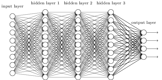
    We've been studying toy networks, with just one neuron in each hidden layer. What about more complex deep networks, with many neurons in each hidden layer?
    tikz40.png

    In fact, much the same behaviour occurs in such networks. In the earlier chapter on backpropagation we saw that the gradient in the llth layer of an LL layer network is given by:

    \[ δ^l=\sum^{′}{(z^l)(w^{l+1})^T}\sum^{′}{(z^{l+1})(w^{l+2})^T}…\sum^{′}{(z^L)∇_aC}\label{124}\tag{124} \]

    Here, \(\sum^{′}{(z^l)\) is a diagonal matrix whose entries are the \(σ′(z)\) values for the weighted inputs to the \(l\)th layer. The \(w^l\) are the weight matrices for the different layers. And \(∇_aC\) is the vector of partial derivatives of \(C\) with respect to the output activations.

    This is a much more complicated expression than in the single-neuron case. Still, if you look closely, the essential form is very similar, with lots of pairs of the form \((w^j)^T\sum^{′}{(z^l)\). What's more, the matrices \(\sum^{′}{(z^l)\) have small entries on the diagonal, none larger than \(1/4\). Provided the weight matrices \(w^j\) aren't too large, each additional term \((w^j)^T\sum^{′}{(z^l)\) tends to make the gradient vector smaller, leading to a vanishing gradient. More generally, the large number of terms in the product tends to lead to an unstable gradient, just as in our earlier example. In practice, empirically it is typically found in sigmoid networks that gradients vanish exponentially quickly in earlier layers. As a result, learning slows down in those layers. This slowdown isn't merely an accident or an inconvenience: it's a fundamental consequence of the approach we're taking to learning.

    Other obstacles to deep learning

    In this chapter we've focused on vanishing gradients - and, more generally, unstable gradients - as an obstacle to deep learning. In fact, unstable gradients are just one obstacle to deep learning, albeit an important fundamental obstacle. Much ongoing research aims to better understand the challenges that can occur when training deep networks. I won't comprehensively summarize that work here, but just want to briefly mention a couple of papers, to give you the flavor of some of the questions people are asking.

    As a first example, in 2010 Glorot and Bengio*

    *Understanding the difficulty of training deep feedforward neural networks, by Xavier Glorot and Yoshua Bengio (2010). See also the earlier discussion of the use of sigmoids in Efficient BackProp, by Yann LeCun, Léon Bottou, Genevieve Orr and Klaus-Robert Müller (1998). found evidence suggesting that the use of sigmoid activation functions can cause problems training deep networks. In particular, they found evidence that the use of sigmoids will cause the activations in the final hidden layer to saturate near \(0\) early in training, substantially slowing down learning. They suggested some alternative activation functions, which appear not to suffer as much from this saturation problem.

    As a second example, in 2013 Sutskever, Martens, Dahl and Hinton*

    *On the importance of initialization and momentum in deep learning, by Ilya Sutskever, James Martens, George Dahl and Geoffrey Hinton (2013). studied the impact on deep learning of both the random weight initialization and the momentum schedule in momentum-based stochastic gradient descent. In both cases, making good choices made a substantial difference in the ability to train deep networks.

    These examples suggest that "What makes deep networks hard to train?" is a complex question. In this chapter, we've focused on the instabilities associated to gradient-based learning in deep networks. The results in the last two paragraphs suggest that there is also a role played by the choice of activation function, the way weights are initialized, and even details of how learning by gradient descent is implemented. And, of course, choice of network architecture and other hyper-parameters is also important. Thus, many factors can play a role in making deep networks hard to train, and understanding all those factors is still a subject of ongoing research. This all seems rather downbeat and pessimism-inducing. But the good news is that in the next chapter we'll turn that around, and develop several approaches to deep learning that to some extent manage to overcome or route around all these challenges.


    This page titled 5.2: Unstable gradients in more complex networks is shared under a CC BY-NC 3.0 license and was authored, remixed, and/or curated by Michael Nielson via source content that was edited to the style and standards of the LibreTexts platform.

    • Was this article helpful?