
6.4: Recent progress in image recognition
- Page ID
- 3776

\( \newcommand{\vecs}[1]{\overset { \scriptstyle \rightharpoonup} {\mathbf{#1}} } \)
\( \newcommand{\vecd}[1]{\overset{-\!-\!\rightharpoonup}{\vphantom{a}\smash {#1}}} \)
\( \newcommand{\id}{\mathrm{id}}\) \( \newcommand{\Span}{\mathrm{span}}\)
( \newcommand{\kernel}{\mathrm{null}\,}\) \( \newcommand{\range}{\mathrm{range}\,}\)
\( \newcommand{\RealPart}{\mathrm{Re}}\) \( \newcommand{\ImaginaryPart}{\mathrm{Im}}\)
\( \newcommand{\Argument}{\mathrm{Arg}}\) \( \newcommand{\norm}[1]{\| #1 \|}\)
\( \newcommand{\inner}[2]{\langle #1, #2 \rangle}\)
\( \newcommand{\Span}{\mathrm{span}}\)
\( \newcommand{\id}{\mathrm{id}}\)
\( \newcommand{\Span}{\mathrm{span}}\)
\( \newcommand{\kernel}{\mathrm{null}\,}\)
\( \newcommand{\range}{\mathrm{range}\,}\)
\( \newcommand{\RealPart}{\mathrm{Re}}\)
\( \newcommand{\ImaginaryPart}{\mathrm{Im}}\)
\( \newcommand{\Argument}{\mathrm{Arg}}\)
\( \newcommand{\norm}[1]{\| #1 \|}\)
\( \newcommand{\inner}[2]{\langle #1, #2 \rangle}\)
\( \newcommand{\Span}{\mathrm{span}}\) \( \newcommand{\AA}{\unicode[.8,0]{x212B}}\)
\( \newcommand{\vectorA}[1]{\vec{#1}} % arrow\)
\( \newcommand{\vectorAt}[1]{\vec{\text{#1}}} % arrow\)
\( \newcommand{\vectorB}[1]{\overset { \scriptstyle \rightharpoonup} {\mathbf{#1}} } \)
\( \newcommand{\vectorC}[1]{\textbf{#1}} \)
\( \newcommand{\vectorD}[1]{\overrightarrow{#1}} \)
\( \newcommand{\vectorDt}[1]{\overrightarrow{\text{#1}}} \)
\( \newcommand{\vectE}[1]{\overset{-\!-\!\rightharpoonup}{\vphantom{a}\smash{\mathbf {#1}}}} \)
\( \newcommand{\vecs}[1]{\overset { \scriptstyle \rightharpoonup} {\mathbf{#1}} } \)
\( \newcommand{\vecd}[1]{\overset{-\!-\!\rightharpoonup}{\vphantom{a}\smash {#1}}} \)
\(\newcommand{\avec}{\mathbf a}\) \(\newcommand{\bvec}{\mathbf b}\) \(\newcommand{\cvec}{\mathbf c}\) \(\newcommand{\dvec}{\mathbf d}\) \(\newcommand{\dtil}{\widetilde{\mathbf d}}\) \(\newcommand{\evec}{\mathbf e}\) \(\newcommand{\fvec}{\mathbf f}\) \(\newcommand{\nvec}{\mathbf n}\) \(\newcommand{\pvec}{\mathbf p}\) \(\newcommand{\qvec}{\mathbf q}\) \(\newcommand{\svec}{\mathbf s}\) \(\newcommand{\tvec}{\mathbf t}\) \(\newcommand{\uvec}{\mathbf u}\) \(\newcommand{\vvec}{\mathbf v}\) \(\newcommand{\wvec}{\mathbf w}\) \(\newcommand{\xvec}{\mathbf x}\) \(\newcommand{\yvec}{\mathbf y}\) \(\newcommand{\zvec}{\mathbf z}\) \(\newcommand{\rvec}{\mathbf r}\) \(\newcommand{\mvec}{\mathbf m}\) \(\newcommand{\zerovec}{\mathbf 0}\) \(\newcommand{\onevec}{\mathbf 1}\) \(\newcommand{\real}{\mathbb R}\) \(\newcommand{\twovec}[2]{\left[\begin{array}{r}#1 \\ #2 \end{array}\right]}\) \(\newcommand{\ctwovec}[2]{\left[\begin{array}{c}#1 \\ #2 \end{array}\right]}\) \(\newcommand{\threevec}[3]{\left[\begin{array}{r}#1 \\ #2 \\ #3 \end{array}\right]}\) \(\newcommand{\cthreevec}[3]{\left[\begin{array}{c}#1 \\ #2 \\ #3 \end{array}\right]}\) \(\newcommand{\fourvec}[4]{\left[\begin{array}{r}#1 \\ #2 \\ #3 \\ #4 \end{array}\right]}\) \(\newcommand{\cfourvec}[4]{\left[\begin{array}{c}#1 \\ #2 \\ #3 \\ #4 \end{array}\right]}\) \(\newcommand{\fivevec}[5]{\left[\begin{array}{r}#1 \\ #2 \\ #3 \\ #4 \\ #5 \\ \end{array}\right]}\) \(\newcommand{\cfivevec}[5]{\left[\begin{array}{c}#1 \\ #2 \\ #3 \\ #4 \\ #5 \\ \end{array}\right]}\) \(\newcommand{\mattwo}[4]{\left[\begin{array}{rr}#1 \amp #2 \\ #3 \amp #4 \\ \end{array}\right]}\) \(\newcommand{\laspan}[1]{\text{Span}\{#1\}}\) \(\newcommand{\bcal}{\cal B}\) \(\newcommand{\ccal}{\cal C}\) \(\newcommand{\scal}{\cal S}\) \(\newcommand{\wcal}{\cal W}\) \(\newcommand{\ecal}{\cal E}\) \(\newcommand{\coords}[2]{\left\{#1\right\}_{#2}}\) \(\newcommand{\gray}[1]{\color{gray}{#1}}\) \(\newcommand{\lgray}[1]{\color{lightgray}{#1}}\) \(\newcommand{\rank}{\operatorname{rank}}\) \(\newcommand{\row}{\text{Row}}\) \(\newcommand{\col}{\text{Col}}\) \(\renewcommand{\row}{\text{Row}}\) \(\newcommand{\nul}{\text{Nul}}\) \(\newcommand{\var}{\text{Var}}\) \(\newcommand{\corr}{\text{corr}}\) \(\newcommand{\len}[1]{\left|#1\right|}\) \(\newcommand{\bbar}{\overline{\bvec}}\) \(\newcommand{\bhat}{\widehat{\bvec}}\) \(\newcommand{\bperp}{\bvec^\perp}\) \(\newcommand{\xhat}{\widehat{\xvec}}\) \(\newcommand{\vhat}{\widehat{\vvec}}\) \(\newcommand{\uhat}{\widehat{\uvec}}\) \(\newcommand{\what}{\widehat{\wvec}}\) \(\newcommand{\Sighat}{\widehat{\Sigma}}\) \(\newcommand{\lt}{<}\) \(\newcommand{\gt}{>}\) \(\newcommand{\amp}{&}\) \(\definecolor{fillinmathshade}{gray}{0.9}\)In 1998, the year MNIST was introduced, it took weeks to train a state-of-the-art workstation to achieve accuracies substantially worse than those we can achieve using a GPU and less than an hour of training. Thus, MNIST is no longer a problem that pushes the limits of available technique; rather, the speed of training means that it is a problem good for teaching and learning purposes. Meanwhile, the focus of research has moved on, and modern work involves much more challenging image recognition problems. In this section, I briefly describe some recent work on image recognition using neural networks.
The section is different to most of the book. Through the book I've focused on ideas likely to be of lasting interest - ideas such as backpropagation, regularization, and convolutional networks. I've tried to avoid results which are fashionable as I write, but whose long-term value is unknown. In science, such results are more often than not ephemera which fade and have little lasting impact. Given this, a skeptic might say: "well, surely the recent progress in image recognition is an example of such ephemera? In another two or three years, things will have moved on. So surely these results are only of interest to a few specialists who want to compete at the absolute frontier? Why bother discussing it?"
Such a skeptic is right that some of the finer details of recent papers will gradually diminish in perceived importance. With that said, the past few years have seen extraordinary improvements using deep nets to attack extremely difficult image recognition tasks. Imagine a historian of science writing about computer vision in the year 2100. They will identify the years 2011 to 2015 (and probably a few years beyond) as a time of huge breakthroughs, driven by deep convolutional nets. That doesn't mean deep convolutional nets will still be used in 2100, much less detailed ideas such as dropout, rectified linear units, and so on. But it does mean that an important transition is taking place, right now, in the history of ideas. It's a bit like watching the discovery of the atom, or the invention of antibiotics: invention and discovery on a historic scale. And so while we won't dig down deep into details, it's worth getting some idea of the exciting discoveries currently being made.
The 2012 LRMD paper: Let me start with a 2012 paper*
*Building high-level features using large scale unsupervised learning, by Quoc Le, Marc'Aurelio Ranzato, Rajat Monga, Matthieu Devin, Kai Chen, Greg Corrado, Jeff Dean, and Andrew Ng (2012). Note that the detailed architecture of the network used in the paper differed in many details from the deep convolutional networks we've been studying. Broadly speaking, however, LRMD is based on many similar ideas. from a group of researchers from Stanford and Google. I'll refer to this paper as LRMD, after the last names of the first four authors. LRMD used a neural network to classify images from ImageNet, a very challenging image recognition problem. The 2011 ImageNet data that they used included 16 million full color images, in 20 thousand categories. The images were crawled from the open net, and classified by workers from Amazon's Mechanical Turk service. Here's a few ImageNet images*
*These are from the 2014 dataset, which is somewhat changed from 2011. Qualitatively, however, the dataset is extremely similar. Details about ImageNet are available in the original ImageNet paper, ImageNet: a large-scale hierarchical image database, by Jia Deng, Wei Dong, Richard Socher, Li-Jia Li, Kai Li, and Li Fei-Fei (2009).:

These are, respectively, in the categories for beading plane, brown root rot fungus, scalded milk, and the common roundworm. If you're looking for a challenge, I encourage you to visit ImageNet's list of hand tools, which distinguishes between beading planes, block planes, chamfer planes, and about a dozen other types of plane, amongst other categories. I don't know about you, but I cannot confidently distinguish between all these tool types. This is obviously a much more challenging image recognition task than MNIST! LRMD's network obtained a respectable \(15.8\) percent accuracy for correctly classifying ImageNet images. That may not sound impressive, but it was a huge improvement over the previous best result of \(9.3\) percent accuracy. That jump suggested that neural networks might offer a powerful approach to very challenging image recognition tasks, such as ImageNet.
The 2012 KSH paper: The work of LRMD was followed by a 2012 paper of Krizhevsky, Sutskever and Hinton (KSH)*
*ImageNet classification with deep convolutional neural networks, by Alex Krizhevsky, Ilya Sutskever, and Geoffrey E. Hinton (2012).
KSH trained and tested a deep convolutional neural network using a restricted subset of the ImageNet data. The subset they used came from a popular machine learning competition - the ImageNet Large-Scale Visual Recognition Challenge (ILSVRC). Using a competition dataset gave them a good way of comparing their approach to other leading techniques. The ILSVRC-2012 training set contained about 1.2 million ImageNet images, drawn from 1,000 categories. The validation and test sets contained 50,000 and 150,000 images, respectively, drawn from the same 1,000 categories.
One difficulty in running the ILSVRC competition is that many ImageNet images contain multiple objects. Suppose an image shows a labrador retriever chasing a soccer ball. The so-called "correct" ImageNet classification of the image might be as a labrador retriever. Should an algorithm be penalized if it labels the image as a soccer ball? Because of this ambiguity, an algorithm was considered correct if the actual ImageNet classification was among the \(5\) classifications the algorithm considered most likely. By this top-\(5\) criterion, KSH's deep convolutional network achieved an accuracy of \(84.7\) percent, vastly better than the next-best contest entry, which achieved an accuracy of \(73.8\) percent. Using the more restrictive metric of getting the label exactly right, KSH's network achieved an accuracy of \(63.3\) percent.
It's worth briefly describing KSH's network, since it has inspired much subsequent work. It's also, as we shall see, closely related to the networks we trained earlier in this chapter, albeit more elaborate. KSH used a deep convolutional neural network, trained on two GPUs. They used two GPUs because the particular type of GPU they were using (an NVIDIA GeForce GTX 580) didn't have enough on-chip memory to store their entire network. So they split the network into two parts, partitioned across the two GPUs.
The KSH network has \(7\) layers of hidden neurons. The first \(5\) hidden layers are convolutional layers (some with max-pooling), while the next \(2\) layers are fully-connected layers. The output layer is a \(1,000\)-unit softmax layer, corresponding to the 1,0001,000 image classes. Here's a sketch of the network, taken from the KSH paper*
*Thanks to Ilya Sutskever.. The details are explained below. Note that many layers are split into \(2\) parts, corresponding to the \(2\) GPUs.
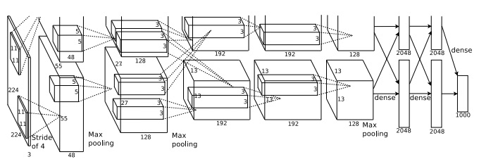
The input layer contains \(3×224×224\) neurons, representing the RGB values for a \(224×224\) image. Recall that, as mentioned earlier, ImageNet contains images of varying resolution. This poses a problem, since a neural network's input layer is usually of a fixed size. KSH dealt with this by rescaling each image so the shorter side had length \(256\). They then cropped out a \(256×256\) area in the center of the rescaled image. Finally, KSH extracted random \(224×224\) subimages (and horizontal reflections) from the \(256×256\) images. They did this random cropping as a way of expanding the training data, and thus reducing overfitting. This is particularly helpful in a large network such as KSH's. It was these \(224×224\) images which were used as inputs to the network. In most cases the cropped image still contains the main object from the uncropped image.
Moving on to the hidden layers in KSH's network, the first hidden layer is a convolutional layer, with a max-pooling step. It uses local receptive fields of size \(11×11\), and a stride length of \(4\) pixels. There are a total of 9696 feature maps. The feature maps are split into two groups of \(48\) each, with the first \(48\) feature maps residing on one GPU, and the second \(48\) feature maps residing on the other GPU. The max-pooling in this and later layers is done in \(3×3\) regions, but the pooling regions are allowed to overlap, and are just \(2\) pixels apart.
The second hidden layer is also a convolutional layer, with a max-pooling step. It uses \(5×5\) local receptive fields, and there's a total of \(256\) feature maps, split into \(128\) on each GPU. Note that the feature maps only use \(48\) input channels, not the full 9696 output from the previous layer (as would usually be the case). This is because any single feature map only uses inputs from the same GPU. In this sense the network departs from the convolutional architecture we described earlier in the chapter, though obviously the basic idea is still the same.
The third, fourth and fifth hidden layers are convolutional layers, but unlike the previous layers, they do not involve max-pooling. Their respectives parameters are: (3) \(384\) feature maps, with \(3×3\) local receptive fields, and \(256\) input channels; (4) \(384\) feature maps, with \(3×3\) local receptive fields, and \(192\) input channels; and (5) \(256\) feature maps, with \(3×3\) local receptive fields, and \(192\) input channels. Note that the third layer involves some inter-GPU communication (as depicted in the figure) in order that the feature maps use all \(256\) input channels.
The sixth and seventh hidden layers are fully-connected layers, with \(4,096\) neurons in each layer.
The output layer is a \(1,000\)-unit softmax layer.
The KSH network takes advantage of many techniques. Instead of using the sigmoid or tanh activation functions, KSH use rectified linear units, which sped up training significantly. KSH's network had roughly 60 million learned parameters, and was thus, even with the large training set, susceptible to overfitting. To overcome this, they expanded the training set using the random cropping strategy we discussed above. They also further addressed overfitting by using a variant of l2 regularization, and dropout. The network itself was trained using momentum-based mini-batch stochastic gradient descent.
That's an overview of many of the core ideas in the KSH paper. I've omitted some details, for which you should look at the paper. You can also look at Alex Krizhevsky's cuda-convnet (and successors), which contains code implementing many of the ideas. A Theano-based implementation has also been developed*
*Theano-based large-scale visual recognition with multiple GPUs, by Weiguang Ding, Ruoyan Wang, Fei Mao, and Graham Taylor (2014)., with the code available here. The code is recognizably along similar lines to that developed in this chapter, although the use of multiple GPUs complicates things somewhat. The Caffe neural nets framework also includes a version of the KSH network, see their Model Zoo for details.
The 2014 ILSVRC competition: Since 2012, rapid progress continues to be made. Consider the 2014 ILSVRC competition. As in 2012, it involved a training set of \(1.2\) million images, in \(1,000\) categories, and the figure of merit was whether the top \(5\) predictions included the correct category. The winning team, based primarily at Google*
*Going deeper with convolutions, by Christian Szegedy, Wei Liu, Yangqing Jia, Pierre Sermanet, Scott Reed, Dragomir Anguelov, Dumitru Erhan, Vincent Vanhoucke, and Andrew Rabinovich (2014)., used a deep convolutional network with 2222 layers of neurons. They called their network GoogLeNet, as a homage to LeNet-5. GoogLeNet achieved a top-5 accuracy of \(93.33\) percent, a giant improvement over the 2013 winner (Clarifai, with \(88.3\) percent), and the 2012 winner (KSH, with \(84.7\) percent).
Just how good is GoogLeNet's \(93.33\) percent accuracy? In 2014 a team of researchers wrote a survey paper about the ILSVRC competition*
*ImageNet large scale visual recognition challenge, by Olga Russakovsky, Jia Deng, Hao Su, Jonathan Krause, Sanjeev Satheesh, Sean Ma, Zhiheng Huang, Andrej Karpathy, Aditya Khosla, Michael Bernstein, Alexander C. Berg, and Li Fei-Fei (2014).
One of the questions they address is how well humans perform on ILSVRC. To do this, they built a system which lets humans classify ILSVRC images. As one of the authors, Andrej Karpathy, explains in an informative blog post, it was a lot of trouble to get the humans up to GoogLeNet's performance:
...the task of labeling images with 5 out of 1000 categories quickly turned out to be extremely challenging, even for some friends in the lab who have been working on ILSVRC and its classes for a while. First we thought we would put it up on [Amazon Mechanical Turk]. Then we thought we could recruit paid undergrads. Then I organized a labeling party of intense labeling effort only among the (expert labelers) in our lab. Then I developed a modified interface that used GoogLeNet predictions to prune the number of categories from 1000 to only about 100. It was still too hard - people kept missing categories and getting up to ranges of 13-15% error rates. In the end I realized that to get anywhere competitively close to GoogLeNet, it was most efficient if I sat down and went through the painfully long training process and the subsequent careful annotation process myself... The labeling happened at a rate of about 1 per minute, but this decreased over time... Some images are easily recognized, while some images (such as those of fine-grained breeds of dogs, birds, or monkeys) can require multiple minutes of concentrated effort. I became very good at identifying breeds of dogs... Based on the sample of images I worked on, the GoogLeNet classification error turned out to be 6.8%... My own error in the end turned out to be 5.1%, approximately 1.7% better.
In other words, an expert human, working painstakingly, was with great effort able to narrowly beat the deep neural network. In fact, Karpathy reports that a second human expert, trained on a smaller sample of images, was only able to attain a \(12.0\) percent top-5 error rate, significantly below GoogLeNet's performance. About half the errors were due to the expert "failing to spot and consider the ground truth label as an option".
These are astonishing results. Indeed, since this work, several teams have reported systems whose top-5 error rate is actually better than 5.1%. This has sometimes been reported in the media as the systems having better-than-human vision. While the results are genuinely exciting, there are many caveats that make it misleading to think of the systems as having better-than-human vision. The ILSVRC challenge is in many ways a rather limited problem - a crawl of the open web is not necessarily representative of images found in applications! And, of course, the top-\(5\) criterion is quite artificial. We are still a long way from solving the problem of image recognition or, more broadly, computer vision. Still, it's extremely encouraging to see so much progress made on such a challenging problem, over just a few years.
Other activity: I've focused on ImageNet, but there's a considerable amount of other activity using neural nets to do image recognition. Let me briefly describe a few interesting recent results, just to give the flavour of some current work.
One encouraging practical set of results comes from a team at Google, who applied deep convolutional networks to the problem of recognizing street numbers in Google's Street View imagery*
*Multi-digit Number Recognition from Street View Imagery using Deep Convolutional Neural Networks, by Ian J. Goodfellow, Yaroslav Bulatov, Julian Ibarz, Sacha Arnoud, and Vinay Shet (2013).In their paper, they report detecting and automatically transcribing nearly 100 million street numbers at an accuracy similar to that of a human operator. The system is fast: their system transcribed all of Street View's images of street numbers in France in less than an hour! They say: "Having this new dataset significantly increased the geocoding quality of Google Maps in several countries especially the ones that did not already have other sources of good geocoding." And they go on to make the broader claim: "We believe with this model we have solved [optical character recognition] for short sequences [of characters] for many applications."
I've perhaps given the impression that it's all a parade of encouraging results. Of course, some of the most interesting work reports on fundamental things we don't yet understand. For instance, a 2013 paper*
*Intriguing properties of neural networks, by Christian Szegedy, Wojciech Zaremba, Ilya Sutskever, Joan Bruna, Dumitru Erhan, Ian Goodfellow, and Rob Fergus (2013) showed that deep networks may suffer from what are effectively blind spots. Consider the lines of images below. On the left is an ImageNet image classified correctly by their network. On the right is a slightly perturbed image (the perturbation is in the middle) which is classified incorrectly by the network. The authors found that there are such "adversarial" images for every sample image, not just a few special ones.

This is a disturbing result. The paper used a network based on the same code as KSH's network - that is, just the type of network that is being increasingly widely used. While such neural networks compute functions which are, in principle, continuous, results like this suggest that in practice they're likely to compute functions which are very nearly discontinuous. Worse, they'll be discontinuous in ways that violate our intuition about what is reasonable behavior. That's concerning. Furthermore, it's not yet well understood what's causing the discontinuity: is it something about the loss function? The activation functions used? The architecture of the network? Something else? We don't yet know.
Now, these results are not quite as bad as they sound. Although such adversarial images are common, they're also unlikely in practice. As the paper notes:
The existence of the adversarial negatives appears to be in contradiction with the network’s ability to achieve high generalization performance. Indeed, if the network can generalize well, how can it be confused by these adversarial negatives, which are indistinguishable from the regular examples? The explanation is that the set of adversarial negatives is of extremely low probability, and thus is never (or rarely) observed in the test set, yet it is dense (much like the rational numbers), and so it is found near virtually every test case.
Nonetheless, it is distressing that we understand neural nets so poorly that this kind of result should be a recent discovery. Of course, a major benefit of the results is that they have stimulated much followup work. For example, one recent paper*
*Deep Neural Networks are Easily Fooled: High Confidence Predictions for Unrecognizable Images, by Anh Nguyen, Jason Yosinski, and Jeff Clune (2014). shows that given a trained network it's possible to generate images which look to a human like white noise, but which the network classifies as being in a known category with a very high degree of confidence. This is another demonstration that we have a long way to go in understanding neural networks and their use in image recognition.
Despite results like this, the overall picture is encouraging. We're seeing rapid progress on extremely difficult benchmarks, like ImageNet. We're also seeing rapid progress in the solution of real-world problems, like recognizing street numbers in StreetView. But while this is encouraging it's not enough just to see improvements on benchmarks, or even real-world applications. There are fundamental phenomena which we still understand poorly, such as the existence of adversarial images. When such fundamental problems are still being discovered (never mind solved), it is premature to say that we're near solving the problem of image recognition. At the same time such problems are an exciting stimulus to further work.