8.7: The sound of sand

Last updated
Save as PDF

Page ID: 46644

\( \newcommand{\vecs}[1]{\overset { \scriptstyle \rightharpoonup} {\mathbf{#1}} } \) \( \newcommand{\vecd}[1]{\overset{-\!-\!\rightharpoonup}{\vphantom{a}\smash {#1}}} \)\(\newcommand{\id}{\mathrm{id}}\) \( \newcommand{\Span}{\mathrm{span}}\) \( \newcommand{\kernel}{\mathrm{null}\,}\) \( \newcommand{\range}{\mathrm{range}\,}\) \( \newcommand{\RealPart}{\mathrm{Re}}\) \( \newcommand{\ImaginaryPart}{\mathrm{Im}}\) \( \newcommand{\Argument}{\mathrm{Arg}}\) \( \newcommand{\norm}[1]{\| #1 \|}\) \( \newcommand{\inner}[2]{\langle #1, #2 \rangle}\) \( \newcommand{\Span}{\mathrm{span}}\) \(\newcommand{\id}{\mathrm{id}}\) \( \newcommand{\Span}{\mathrm{span}}\) \( \newcommand{\kernel}{\mathrm{null}\,}\) \( \newcommand{\range}{\mathrm{range}\,}\) \( \newcommand{\RealPart}{\mathrm{Re}}\) \( \newcommand{\ImaginaryPart}{\mathrm{Im}}\) \( \newcommand{\Argument}{\mathrm{Arg}}\) \( \newcommand{\norm}[1]{\| #1 \|}\) \( \newcommand{\inner}[2]{\langle #1, #2 \rangle}\) \( \newcommand{\Span}{\mathrm{span}}\)\(\newcommand{\AA}{\unicode[.8,0]{x212B}}\)

As my implementation of SandPile runs, it records the number of cells that topple during each time step, accumulating the results in a list called toppled_seq. After running the model in Section 8.4, we can extract the resulting signal:

signal = pile2.toppled_seq

To compute the power spectrum of this signal we can use the SciPy function welch:

from scipy.signal import welch 

nperseg = 2048 
freqs, spectrum = welch(signal, nperseg=nperseg, fs=nperseg)

This function uses Welch’s method, which splits the signal into segments and computes the power spectrum of each segment. The result is typically noisy, so Welch’s method averages across segments to estimate the average power at each frequency. For more about Welch’s method, see http://thinkcomplex.com/welch.

The parameter nperseg specifies the number of time steps per segment. With longer segments, we can estimate the power for more frequencies. With shorter segments, we get better estimates for each frequency. The value I chose, 2048, balances these tradeoffs.

The parameter fs is the “sampling frequency”, which is the number of data points in the signal per unit of time. By setting fs=nperseg, we get a range of frequencies from 0 to nperseg/2. This range is convenient, but because the units of time in the model are arbitrary, it doesn’t mean much.

The return values, freqs and powers, are NumPy arrays containing the frequencies of the components and their corresponding powers, which we can plot. Figure \(\PageIndex{1}\) shows the result.

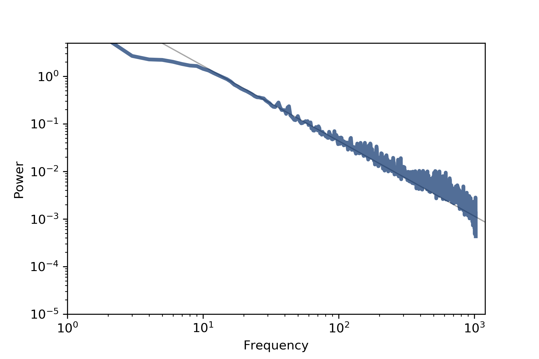
Figure \(\PageIndex{1}\): Power spectrum of the number of toppled cells over time, log-log scale.

For frequencies between 10 and 1000 (in arbitrary units), the spectrum falls on a straight line, which is what we expect for pink or red noise.

The gray line in the figure has slope −1.58, which indicates that

\[\log P(f) ∼ −β \log f \nonumber\]

with parameter β=1.58, which is the same parameter reported by Bak, Tang, and Wiesenfeld. This result confirms that the sand pile model generates pink noise.