10.2: Solving Systems of ODEs

Now that we’ve seen the basics of matrices, let’s see how we can use them to solve systems of differential equations.

Lotka-Volterra

The Lotka-Volterra model describes the interactions between two species in an ecosystem, a predator and its prey. As an example, we’ll consider foxes and rabbits.

The model is governed by the following system of differential equations:

\[\begin{aligned} \frac{dx}{dt} = a x - b x y \\ \frac{dy}{dt} = -c y + d x y\end{aligned}\]

where \(x\) and \(y\) are the populations of rabbits and foxes, and \(a\), \(b\), \(c\), and \(d\) are parameters that quantify the interactions between the two species (see https://greenteapress.com/matlab/lotka).

At first glance, you might think you could solve these equations by calling ode45 once to solve for \(x\) and once to solve for \(y\). The problem is that each equation involves both variables, which is what makes this a system of equations and not just a list of unrelated equations. To solve a system, you have to solve the equations simultaneously.

Fortunately, ode45 can handle systems of equations. The difference is that the initial condition is a vector that contains the initial values \(x(0)\) and \(y(0)\), and the output is a matrix that contains one column for \(x\) and one for \(y\).

Listing 10.1 shows the rate function with the parameters \(a = 0.1\), \(b = 0.01\), \(c = 0.1\), and \(d = 0.002\):

Listing 10.1: A rate function for Lotka-Volterra

function res = rate_func(t, V)
    % unpack the elements of V
    x = V(1);
    y = V(2);

    % set the parameters
    a = 0.1;
    b = 0.01;
    c = 0.1;
    d = 0.002;

    % compute the derivatives
    dxdt = a*x - b*x*y;
    dydt = -c*y + d*x*y;

    % pack the derivatives into a vector
    res = [dxdt; dydt];
end

The first input variable, t, is time. Even though the time variable is not used in this rate function, it has to be there in order for this function to work with ode45. The second input variable, V, is a vector with two elements, \(x(t)\) and \(y(t)\). The body of the function includes four sections, each explained by a comment.

The first section unpacks the vector by copying the elements into variables. This isn’t necessary, but giving names to these values will help you to remember what’s what. It also makes the third section, where we compute the derivatives, resemble the mathematical equations we were given, which helps prevent errors.

The second section sets the parameters that describe the reproductive rates of rabbits and foxes, and the characteristics of their interactions. If we were studying a real system, these values would come from observations of real animals, but for this example I chose values that yield interesting results.

The third section computes the derivatives of \(x\) and \(y\), using the equations we were given.

The last section packs the computed derivatives back into a vector. When ode45 calls this function, it provides a vector as input and expects to get a vector as output.

Sharp-eyed readers will notice something different about this line:

    res = [drdt; dfdt];

The semicolon between the elements of the vector is not an error. It is necessary in this case because ode45 requires the result of this function to be a column vector.

As always, it’s a good idea to test your rate function before you call ode45. Create a file named lotka.m with the following top-level function:

function res = lotka()
    t = 0;
    V_init = [80, 20];
    rate_func(t, V_init)
end

V_init is a vector that represents the initial condition, 80 rabbits and 20 foxes. The result from rate_func is

-8.0000
 1.2000
 

which means that with these initial conditions, we expect the rabbit population to decline initially at a rate of 8 per week and the fox population to increase by 1.2 per week.

Now we can run ode45 like this:

tspan = [0, 200]
[T, M] = ode45(@rate_func, tspan, V_init)

The first argument is the function handle for the rate function. The second argument is the time span, from 0 to 200 weeks. The third argument is the initial condition.

Output Matrices

The ode45 function returns two values: T, a vector, and M, a matrix.

>> size(T)
ans = 101     1

>> size(M)
ans = 101     2

T has 101 rows and 1 column, so it is a column vector with one row for each time step.

M has 101 rows, one for each time step, and 2 columns, one for each variable, \(x\) and \(y\).

This structure—one column per variable—is a common way to use matrices. And plot understands this structure, so if you do the following:

>> plot(T, M)

MATLAB understands that it should plot each column from M versus T.

You can copy the columns of M into other variables like this:

>> R = M(:, 1);
>> F = M(:, 2);

In this context, the colon represents the range from 1 to end, so M(:, 1) means “all the rows, column 1” and M(:, 2) means “all the rows, column 2.”

>> size(R)
ans = 101     1

>> size(F)
ans = 101     1

So R and F are column vectors.

Now we can plot these vectors separately, which makes it easier to give them different style strings:

>> plot(T, R, '-')
>> plot(T, F, '--')

Figure 10.1 shows the results. The x-axis is time in weeks; the y-axis is population. The top curve shows the population of rabbits; the bottom curve shows foxes.

Figure 10.1: Solution for the Lotka-Volterra model

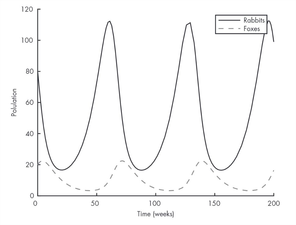
Initially, there are too many foxes, so the rabbit population declines. Then there are not enough rabbits, and the fox population declines. That allows the rabbit population to recover, and the pattern repeats.

This cycle of “boom and bust” is typical of the Lotka-Volterra model.

Phase Plot

Instead of plotting the two populations over time, it is sometimes useful to plot them against each other:

>> plot(R, F)

Figure 10.2 shows the result, which is called a phase plot. Each point on this plot represents a certain number of rabbits (on the x-axis) and a certain number of foxes (on the y-axis). Since these are the only two variables in the system, each point in this plane describes the complete state of the system, that is, the values of the variables we’re solving for.

Figure 10.2: Phase plot from the Lotka-Volterra model

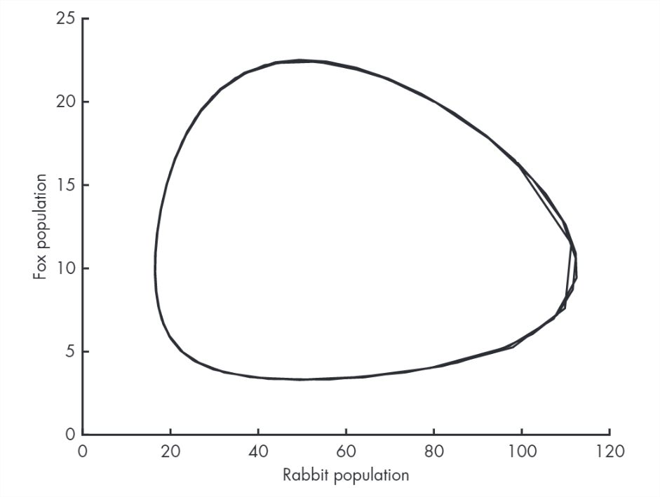
Over time, the state moves around the plane. Figure 10.2 shows the path traced by the state over time; this path is called a trajectory.

Since the behavior of this system is periodic, the trajectory is a loop.

If there are three variables in the system, we need three dimensions to show the state of the system, so the trajectory is a 3D curve. You can use plot3 to trace trajectories in three dimensions, but for four or more variables, you’re on your own.

What Could Go Wrong?

The output vector from the rate function has to be a column vector, otherwise you get an error:

Error using odearguments (line 93)
RATE_FUNC must return a column vector.

which is a pretty good error message. It’s not clear why it needs to be a column vector, but that’s not our problem.

Another possible error is reversing the order of the elements in the initial conditions or the vectors inside lotka. MATLAB doesn’t know what the elements are supposed to mean, so it can’t catch errors like this; it will just produce incorrect results.

The order of the elements (rabbits and foxes) is up to you, but you have to be consistent. That is, the order of the initial conditions you provide when you call ode45 has to be the same as the order inside rate_func where you unpack the input vector and the same as the order of the derivatives in the output vector.