11.2: Free Fall

As an example of Newtonian motion, let’s go back to the question from Section 1.1:

If you drop a penny from the top of the Empire State Building, how long does it take to reach the sidewalk, and how fast is it going when it gets there?

We’ll start with no air resistance; then we’ll add air resistance to the model and see what effect it has.

Near the surface of the earth, acceleration due to gravity is -9.8 m/s², where the minus sign indicates that gravity pulls down. If the object falls straight down, we can describe its position with a scalar value \(y\), representing altitude.

Listing 11.1 contains a rate function we can use with ode45 to solve this problem:

Listing 11.1: A rate function for the falling penny problem

function res = rate_func(t, X)
    % unpack position and velocity
    y = X(1);
    v = X(2);

    % compute the derivatives
    dydt = v;
    dvdt = -9.8;

    % pack the derivatives into a column vector
    res = [dydt; dvdt];
end

The rate function in Listing 11.1 takes t and X as input variables, where the elements of X are understood to be the position and velocity of the penny.

It returns a column vector that contains dydt and dvdt, which are velocity and acceleration, respectively. Since velocity is the second element of X, we can simply assign this value to dydt. And since the derivative of velocity is acceleration, we can assign the acceleration due to gravity to dvdt.

As always, we should test the rate function before we call ode45. Here’s the top-level function we can use to test it:

function penny()
   t = 0;
   X = [381, 0];
   rate_func(t, X)
end

The initial condition of X is the initial position, which is the height of the Empire State Building, about 381 m, and the initial velocity, which is 0 m/s.

The result from rate_func is

    0
   -9.8000

which is what we expect.

Now we can run ode45 with this rate function:

tspan = [0, 10]
[T, M] = ode45(@rate_func, tspan, X)

As always, the first argument is the function handle, the second is the time span (10 seconds), and the third is the initial condition.

The result is a vector, T, that contains the time values, and a matrix, M, that contains two columns, one for altitude and one for velocity.

We can extract the first column and plot it, like this:

Y = M(:, 1)
plot(T, Y)

Figure 11.1: Altitude versus time for an object in free fall

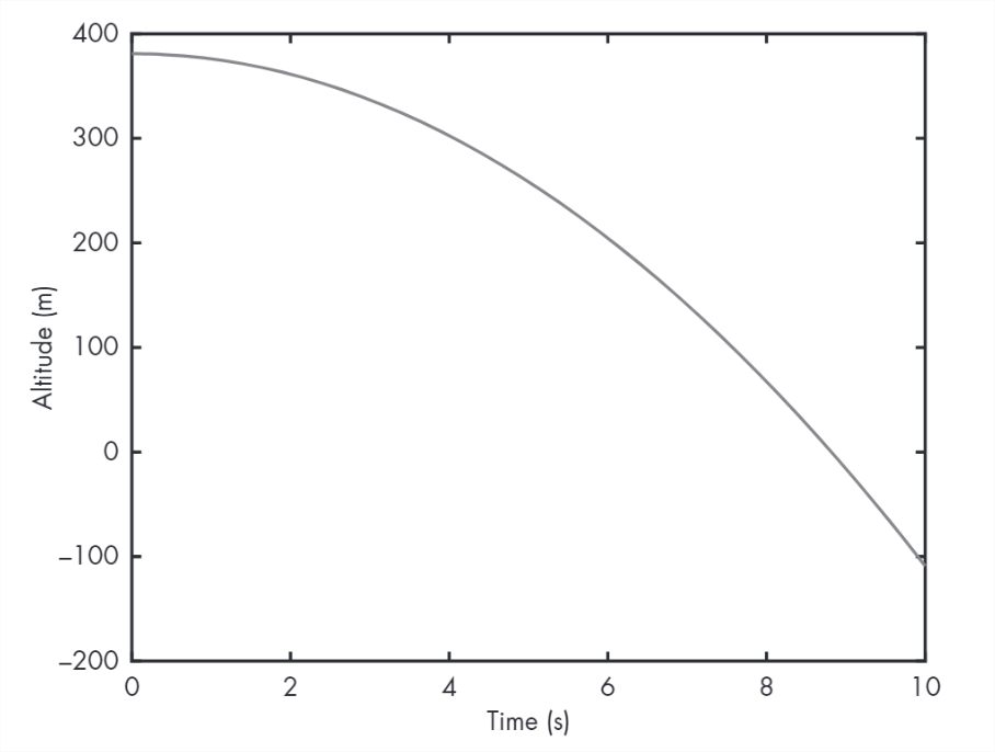
Figure 11.1 shows the result. Altitude drops slowly at first and picks up speed. Between 8 and 9 seconds, the altitude reaches 0, which means the penny hits the sidewalk. But ode45 doesn’t know where the ground is, so the penny keeps going through 0 into negative altitude. We’ll solve that problem in the next section.