15.1: How ode45 Works

Last updated
Save as PDF

Page ID: 84552

\( \newcommand{\vecs}[1]{\overset { \scriptstyle \rightharpoonup} {\mathbf{#1}} } \) \( \newcommand{\vecd}[1]{\overset{-\!-\!\rightharpoonup}{\vphantom{a}\smash {#1}}} \)\(\newcommand{\id}{\mathrm{id}}\) \( \newcommand{\Span}{\mathrm{span}}\) \( \newcommand{\kernel}{\mathrm{null}\,}\) \( \newcommand{\range}{\mathrm{range}\,}\) \( \newcommand{\RealPart}{\mathrm{Re}}\) \( \newcommand{\ImaginaryPart}{\mathrm{Im}}\) \( \newcommand{\Argument}{\mathrm{Arg}}\) \( \newcommand{\norm}[1]{\| #1 \|}\) \( \newcommand{\inner}[2]{\langle #1, #2 \rangle}\) \( \newcommand{\Span}{\mathrm{span}}\) \(\newcommand{\id}{\mathrm{id}}\) \( \newcommand{\Span}{\mathrm{span}}\) \( \newcommand{\kernel}{\mathrm{null}\,}\) \( \newcommand{\range}{\mathrm{range}\,}\) \( \newcommand{\RealPart}{\mathrm{Re}}\) \( \newcommand{\ImaginaryPart}{\mathrm{Im}}\) \( \newcommand{\Argument}{\mathrm{Arg}}\) \( \newcommand{\norm}[1]{\| #1 \|}\) \( \newcommand{\inner}[2]{\langle #1, #2 \rangle}\) \( \newcommand{\Span}{\mathrm{span}}\)\(\newcommand{\AA}{\unicode[.8,0]{x212B}}\)

According to the MATLAB documentation, ode45 uses “an explicit Runge-Kutta formula, the Dormand-Prince pair.” You can read about it at https://greenteapress.com/matlab/runge, but I’ll give you a sense of it here.

The key idea behind all Runge-Kutta methods is to evaluate the rate function several times at each time step and use a weighted average of the computed slopes to estimate the value at the next time step. Different methods evaluate the rate function in different places and compute the average with different weights.

As an example, we’ll solve the following differential equation:

\[\frac{dy}{dt}(t) = y \sin t \notag\]

Given a differential equation, it’s usually straightforward to write a rate function:

function res = rate_func(t, y)
    dydt = y * sin(t);
    res = dydt;
end

And we can use it like this:

    y0 = 1;
    tspan=[0 4];
    options = odeset('Refine', 1);
    [T, Y] = ode45(@rate_func, tspan, y0, options);

For this example we’ll use odeset to set the Refine option to 1, which tells ode45 to return only the time steps it computes, rather than interpolating between them.

Now we can modify the rate function to plot the places where it gets evaluated:

function res = rate_func(t, y)
    dydt = y * sin(t);
    res = dydt;

    plot(t, y, 'ro')
    dt = 0.01;
    ts = [t t+dt];
    ys = [y y+dydt*dt];
    plot(ts, ys, 'r-')
end

When rate_func runs, it plots a red circle at each location and a short red line showing the computed slope.

Figure 15.1 shows the result; ode45 computes 10 time steps (not counting the initial condition) and evaluates the rate function 61 times.

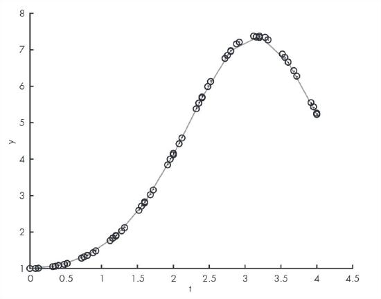
15.1.jpg — Figure 15.1: Points where `ode45` evaluates the rate function

Figure 15.2 shows the same plot, zoomed in on a single time step. The dark squares at \(0.8\) to \(1.2\) show the values that were returned as part of the solution. The circles show the places where the rate function was evaluated.

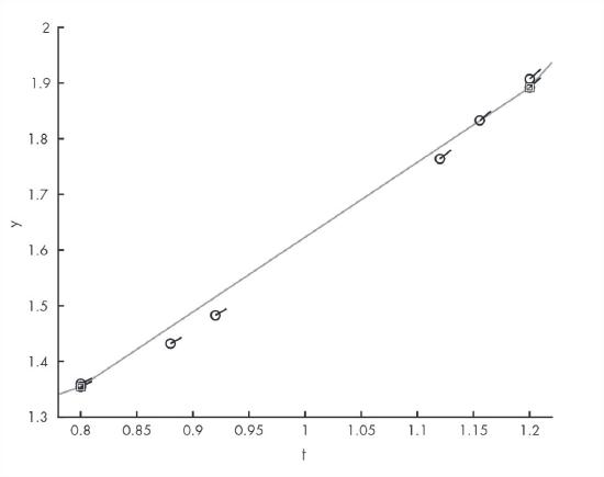
15.2.jpg — Figure 15.2: Points where `ode45` evaluates the rate function, zoomed in

We can see that ode45 evaluates the rate function several times per time step, at several places between the end points. We can also see that most of the places where ode45 evaluates the rate function are not part of the solution it returns, and they are not always good estimates of the solution. This is good to know when you are writing a rate function; you should not assume that the time and state you get as input variables will be part of the solution.

In a sense, the rate function is answering a hypothetical question: “If the state at a particular time has these particular values, what would the slope be?”

At each time step, ode45 actually computes two estimates of the next value. By comparing them, it can estimate the magnitude of the error, which it uses to adjust the time step. If the error is too big, it uses a smaller time step; if the error is small enough, it uses a bigger time step. Because ode45 is adaptive in this way, it minimizes the number of times it calls the rate function to achieve a given level of accuracy.