3.3: Weight initialization

When we create our neural networks, we have to make choices for the initial weights and biases. Up to now, we've been choosing them according to a prescription which I discussed only briefly back in Chapter 1. Just to remind you, that prescription was to choose both the weights and biases using independent Gaussian random variables, normalized to have mean \(0\) and standard deviation \(1\). While this approach has worked well, it was quite ad hoc, and it's worth revisiting to see if we can find a better way of setting our initial weights and biases, and perhaps help our neural networks learn faster.

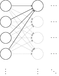
It turns out that we can do quite a bit better than initializing with normalized Gaussians. To see why, suppose we're working with a network with a large number - say \(1,000\) - of input neurons. And let's suppose we've used normalized Gaussians to initialize the weights connecting to the first hidden layer. For now I'm going to concentrate specifically on the weights connecting the input neurons to the first neuron in the hidden layer, and ignore the rest of the network:

We'll suppose for simplicity that we're trying to train using a training input \(x\) in which half the input neurons are on, i.e., set to \(1\), and half the input neurons are off, i.e., set to \(0\). The argument which follows applies more generally, but you'll get the gist from this special case. Let's consider the weighted sum \(z=\sum_j{w_jx_j+b}\) of inputs to our hidden neuron. \(500\) terms in this sum vanish, because the corresponding input \(x_j\) is zero. And so \(z\) is a sum over a total of \(501\) normalized Gaussian random variables, accounting for the \(500\) weight terms and the \(1\) extra bias term. Thus \(z\) is itself distributed as a Gaussian with mean zero and standard deviation \(\sqrt{501}≈22.4\).That is, \(z\) has a very broad Gaussian distribution, not sharply peaked at all:

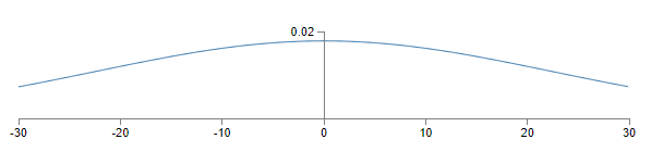
In particular, we can see from this graph that it's quite likely that \(|z|\) will be pretty large, i.e., either \(z≫1\) or \(z≪−1\). If that's the case then the output \(σ(z)\) from the hidden neuron will be very close to either \(1\) or \(0\). That means our hidden neuron will have saturated. And when that happens, as we know, making small changes in the weights will make only absolutely miniscule changes in the activation of our hidden neuron. That miniscule change in the activation of the hidden neuron will, in turn, barely affect the rest of the neurons in the network at all, and we'll see a correspondingly miniscule change in the cost function. As a result, those weights will only learn very slowly when we use the gradient descent algorithm*

*We discussed this in more detail in Chapter 2, where we used the equations of backpropagation to show that weights input to saturated neurons learned slowly.

It's similar to the problem we discussed earlier in this chapter, in which output neurons which saturated on the wrong value caused learning to slow down. We addressed that earlier problem with a clever choice of cost function. Unfortunately, while that helped with saturated output neurons, it does nothing at all for the problem with saturated hidden neurons.

I've been talking about the weights input to the first hidden layer. Of course, similar arguments apply also to later hidden layers: if the weights in later hidden layers are initialized using normalized Gaussians, then activations will often be very close to \(0\) or \(1\), and learning will proceed very slowly.

Is there some way we can choose better initializations for the weights and biases, so that we don't get this kind of saturation, and so avoid a learning slowdown? Suppose we have a neuron with \(n_{in}\) input weights. Then we shall initialize those weights as Gaussian random variables with mean \(0\) and standard deviation \(1/\sqrt{n_{in}}\). That is, we'll squash the Gaussians down, making it less likely that our neuron will saturate. We'll continue to choose the bias as a Gaussian with mean \(0\) and standard deviation \(1\), for reasons I'll return to in a moment. With these choices, the weighted sum \(z=\sum_j{w_jx_j+b}\) will again be a Gaussian random variable with mean \(0\), but it'll be much more sharply peaked than it was before. Suppose, as we did earlier, that \(500\) of the inputs are zero and \(500\) are \(1\). Then it's easy to show (see the exercise below) that \(z\) has a Gaussian distribution with mean \(0\) and standard deviation \(\sqrt{3/2}=1.22\)…. This is much more sharply peaked than before, so much so that even the graph below understates the situation, since I've had to rescale the vertical axis, when compared to the earlier graph:

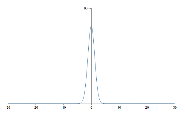
Such a neuron is much less likely to saturate, and correspondingly much less likely to have problems with a learning slowdown.

Exercise

• Verify that the standard deviation of \(z=\sum_j{w_jx_j+b}\) in the paragraph above is \(\sqrt{3/2}\). It may help to know that: (a) the variance of a sum of independent random variables is the sum of the variances of the individual random variables; and (b) the variance is the square of the standard deviation.

I stated above that we'll continue to initialize the biases as before, as Gaussian random variables with a mean of \(0\) and a standard deviation of \(1\). This is okay, because it doesn't make it too much more likely that our neurons will saturate. In fact, it doesn't much matter how we initialize the biases, provided we avoid the problem with saturation. Some people go so far as to initialize all the biases to \(0\), and rely on gradient descent to learn appropriate biases. But since it's unlikely to make much difference, we'll continue with the same initialization procedure as before.

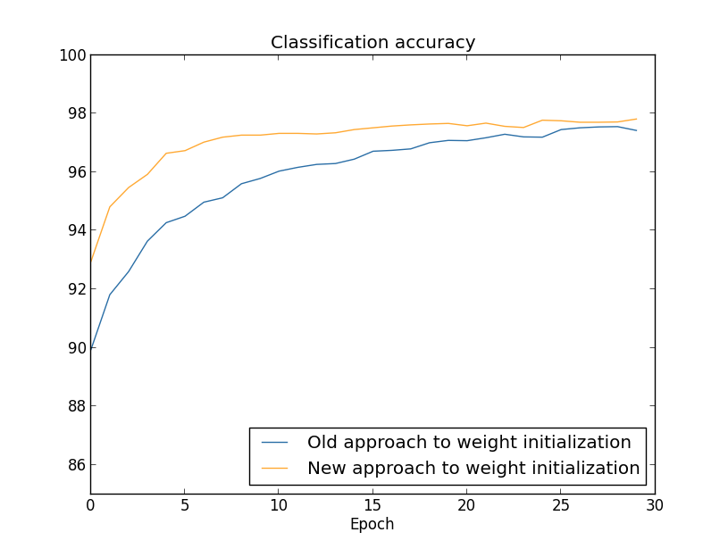
Let's compare the results for both our old and new approaches to weight initialization, using the MNIST digit classification task. As before, we'll use \(30\) hidden neurons, a mini-batch size of \(10\), a regularization parameter \(λ=5.0\), and the cross-entropy cost function. We will decrease the learning rate slightly from \(η=0.5\) to \(0.1\), since that makes the results a little more easily visible in the graphs. We can train using the old method of weight initialization:

>>> import mnist_loader
>>> training_data, validation_data, test_data = \
... mnist_loader.load_data_wrapper()
>>> import network2
>>> net = network2.Network([784, 30, 10], cost=network2.CrossEntropyCost)
>>> net.large_weight_initializer()
>>> net.SGD(training_data, 30, 10, 0.1, lmbda = 5.0,
... evaluation_data=validation_data, 
... monitor_evaluation_accuracy=True)

We can also train using the new approach to weight initialization. This is actually even easier, since network2's default way of initializing the weights is using this new approach. That means we can omit the net.large_weight_initializer() call above:

>>> net = network2.Network([784, 30, 10], cost=network2.CrossEntropyCost)
>>> net.SGD(training_data, 30, 10, 0.1, lmbda = 5.0,
... evaluation_data=validation_data, 
... monitor_evaluation_accuracy=True)

Plotting the results**The program used to generate this and the next graph is weight_initialization.py., we obtain:

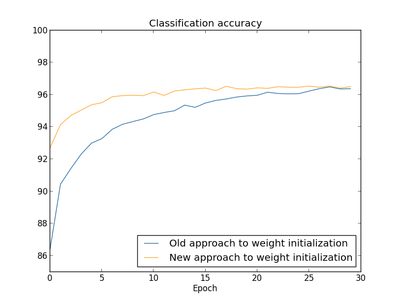
In both cases, we end up with a classification accuracy somewhat over \(96\) percent. The final classification accuracy is almost exactly the same in the two cases. But the new initialization technique brings us there much, much faster. At the end of the first epoch of training the old approach to weight initialization has a classification accuracy under \(87\) percent, while the new approach is already almost \(93\) percent. What appears to be going on is that our new approach to weight initialization starts us off in a much better regime, which lets us get good results much more quickly. The same phenomenon is also seen if we plot results with \(100\) hidden neurons:

In this case, the two curves don't quite meet. However, my experiments suggest that with just a few more epochs of training (not shown) the accuracies become almost exactly the same. So on the basis of these experiments it looks as though the improved weight initialization only speeds up learning, it doesn't change the final performance of our networks. However, in Chapter 4 we'll see examples of neural networks where the long-run behaviour is significantly better with the \(1/\sqrt{n_{in}}\) weight initialization. Thus it's not only the speed of learning which is improved, it's sometimes also the final performance.

The \(1/\sqrt{n_{in}}\) approach to weight initialization helps improve the way our neural nets learn. Other techniques for weight initialization have also been proposed, many building on this basic idea. I won't review the other approaches here, since \(1/\sqrt{n_{in}}\) works well enough for our purposes. If you're interested in looking further, I recommend looking at the discussion on pages 14 and 15 of a 2012 paper by Yoshua Bengio*

*Practical Recommendations for Gradient-Based Training of Deep Architectures, by Yoshua Bengio (2012)., as well as the references therein.

Problem

• Connecting regularization and the improved method of weight initialization L2 regularization sometimes automatically gives us something similar to the new approach to weight initialization. Suppose we are using the old approach to weight initialization. Sketch a heuristic argument that: (1) supposing \(λ\) is not too small, the first epochs of training will be dominated almost entirely by weight decay; (2) provided \(ηλ≪n\) the weights will decay by a factor of \(exp(−ηλ/m)\) per epoch; and (3) supposing \(λ\) is not too large, the weight decay will tail off when the weights are down to a size around \(1/\sqrt{n}\), where \(n\) is the total number of weights in the network. Argue that these conditions are all satisfied in the examples graphed in this section.