3.1: Activity 1 - Data Structures

Introduction

This section introduces the learner to the different data structures that are used to organize data in the computer. Better data organization ensures efficient utilization of the computer. These include arrays, lists, linked lists, stacks, queues, hashing and trees. The different data structures offer advantages to algorithm designers in that they are able to know which one would enable efficient use of the computer.

Definition of Data Structures

Data structures are a particular way of organizing data in the computer in order to be used efficiently. It is defined as an arrangement of data in memory locations to represent values of the carrier set of an abstract data type. Different structures are best suited to different kinds of applications in the computer. Others are even highly specialized to specific tasks. A good example is like in databases which use the B-tree indexes for small percentages of data retrieval and compilers. Another example in databases is the use of dynamic hash tables as look up tables. Data structures also provide a means to manage large amounts of data efficiently for uses such as in large databases and internet indexing services. Efficient data structures are key to designing efficient algorithms.

Data structures are based on the ability of a computer to fetch and store data at any place in its memory, which is normally specified by a pointer – a bit string, representing a memory address that can be itself stored in memory and manipulated by the program.

Examples of data structures consist of:

1. Array

An array is said to be a fixed length, ordered collection of values of the same type stored in contiguous memory locations. The collection may be ordered in several dimensions. An array consists of a collection of elements (values or variables), each identified by at least one array index or key. An array can be considered as the simplest type of data structure, and can be either a one-dimensional array or a two-dimensional array (matrices). Arrays are used to implement tables, especially lookup tables and also lists and strings used by almost every program in the computer. They effectively exploit the addressing logic of computers. In most modern computers and many external storage devices, the memory is a one-dimensional array of words, whose indices are their addresses. Processors, especially vector processors, are often optimized for array operations.

The ability to compute the element indices at run time makes arrays important and useful. This feature allows a single iterative statement to process arbitrarily many elements of an array. This is because, the elements of an array data structure are required to have the same size and should use the same data representation.

2. Lists

A list is defined as an abstract data type that represents a sequence of values, where the same value may occur more than once. An instance of a list is a computer representation of the mathematical concept of a finite sequence; the (potentially) infinite analog of a list is a stream. They are a basic example of containers, as they contain other values. There are two families of lists. Those that primarily expose an infrastructure for the first element, and the rest of the elements, and one whose primary interface is random access through an indexer.

Figure \(\PageIndex{1}\): A list representation

Many programming languages provide support for list data types, and have special syntax and semantics for lists and list operations. A list can often be constructed by writing the items in sequence, separated by commas, semicolons, or spaces, within a pair of delimiters such as parentheses ‘()’, brackets ‘[]’, braces ‘{}’, or angle brackets ‘<>’.

3. Linked Lists

​​​​​​​A linked list is a data structure that consists of a group of nodes which together represent a sequence. Under the simplest form, each node is composed of a data and a reference (a link) to the next node in the sequence; more complex variants add additional links. This structure allows for efficient insertion or removal of elements from any position in the sequence.

Figure \(\PageIndex{2}\): A linked list

They are among the simplest and most common data structures and which can be used to implement several other common abstract data types. They have the principal benefit over a conventional array in that the list elements can easily be inserted or removed. This can be done without reallocation or reorganization of the entire structure as the data items need not be stored contiguously in memory or on disk. On the other hand, an array has to be declared in the source code, before compiling and running the program. They allow insertion and removal of nodes at any point in the list, and can do so with a constant number of operations if the link previous to the link being added or removed is maintained during list traversal. It has the following advantages and disadvantages:

Advantages:

• It is a dynamic data structure, allocating the needed memory while the program is running.
• Insertion and deletion node operations are easily implemented in a linked list.
• Linear data structures such as stacks and queues are easily executed with a linked list.
• They can reduce access time and may expand in real time without memory overhead.

Disadvantages:

• They have a tendency to waste memory due to pointers requiring extra storage space.
• Nodes in a linked list must be read in order from the beginning as linked lists are inherently sequential access.
• Nodes are stored incontiguously, greatly increasing the time required to access individual elements within the list.
• Difficulties arise in linked lists when it comes to reverse traversing. Singly linked lists are extremely difficult to navigate backwards, and while doubly linked lists are somewhat easier to read, memory is wasted in allocating space for a back pointer.

4. Stack

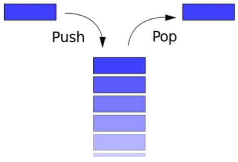
This is a particular kind of abstract data type or collection in which the principal operations on the collection are the addition of an entity to the collection (push) and removal of an entity (pop).

Figure \(\PageIndex{3}\): A diagram of a stack

The stack is a Last-In-First-Out (LIFO) data structure, i.e. the last element added to the structure must be the first one to be removed. The push and pop operations occur only at one end of the structure, referred to as the top of the stack. A peek or top operation can also be implemented, returning the value of the top element without removing it.

A stack is said to be full if it does not contain enough space to accept an entity to be pushed, and it is then considered to be in an overflow state. A pop operation removes an item from the top of the stack. A stack is a restricted data structure, because only a small number of operations are performed on it. The nature of the pop and push operations also mean that stack elements have a natural order. Elements are removed from the stack in the reverse order to the order of their addition.

5. Queues

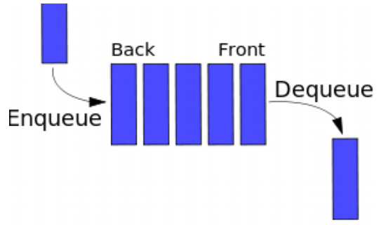
A queue is a kind of abstract data type or collection in which the entities in the collection are kept in order and the principal operations on the collection are the addition of entities to the rear terminal position, and removal of entities from the front terminal position. It is a First-In-First-Out (FIFO) data structure. In a FIFO data structure, the first element added to the queue will be the first one to be removed. It is an example of a linear data structure.

Figure \(\PageIndex{4}\): A diagram of a queue

6. Hashing

Hashing is a method for storing and retrieving records from a database. Hashing allows one to insert, delete, and search for records based on a search key value. A hash system stores records in an array called a hash table. It works by performing a computation on a search key K in a way that is intended to identify the position in hash table that contains the record with key K.

The calculations are done by a function called the hash function. Hash function is any function that can be used to map digital data of arbitrary size to digital data of fixed size, with slight differences in input data producing very big differences in output data. Since hashing schemes place records in the table in whatever order satisfies the needs of the address calculation, records are not ordered by value. A position in the hash table is known as a slot. The number of slots in hash table will be denoted by the variable M with slots numbered from 0 to M - 1.

Hashing is used to index and retrieve items in a database, it is faster to find the item using the shorter hashed key than to find it using the original value. It is also used in many encryption algorithms, and also to encrypt and decrypt digital signatures.

7. Trees

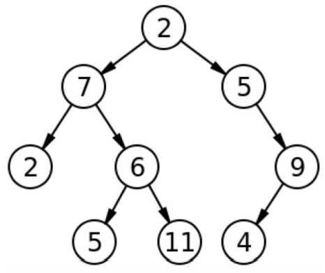
​​​​​​​A tree is a data structure made up of nodes or vertices and edges without having any cycle. A tree with no nodes is called the null or empty tree. A tree that is not empty consists of a root node and potentially many levels of additional nodes that form a hierarchy.

In computer science, it is a widely used abstract data type (ADT) or data structure implementing this ADT that simulates a hierarchical tree structure, with a root value and subtrees of children, represented as a set of linked nodes.

A tree data structure can be defined recursively as a collection of nodes (starting at a root node), where each node is a data structure consisting of a value, together with a list of references to nodes (the “children”), with the constraints that no reference is duplicated, and none points to the root.

Figure \(\PageIndex{5}\): Diagram of a tree

Conclusion

This activity section has introduced the learner to the different data structures used to organize data in the memory of the computer, to make it efficient. It has also highlighted a few examples where they apply. Cited cases include the use of B-trees indexing in the databases and use of hashing to index and retrieve data in a database among others. The data structures looked at in this unit include: Arrays, Lists, Linked lists, Stack, Queues, Hashing and Trees.

Assessment

1. Differentiate between a queue and a stack data structures.
2. Define linear data structures and give an example.
3. List out the basic operations that can be performed on a stack.
4. Briefly state the difference between queues and linked lists.