
12.1: Representing a Graph by a Matrix
- Page ID
- 8485

\( \newcommand{\vecs}[1]{\overset { \scriptstyle \rightharpoonup} {\mathbf{#1}} } \)
\( \newcommand{\vecd}[1]{\overset{-\!-\!\rightharpoonup}{\vphantom{a}\smash {#1}}} \)
\( \newcommand{\id}{\mathrm{id}}\) \( \newcommand{\Span}{\mathrm{span}}\)
( \newcommand{\kernel}{\mathrm{null}\,}\) \( \newcommand{\range}{\mathrm{range}\,}\)
\( \newcommand{\RealPart}{\mathrm{Re}}\) \( \newcommand{\ImaginaryPart}{\mathrm{Im}}\)
\( \newcommand{\Argument}{\mathrm{Arg}}\) \( \newcommand{\norm}[1]{\| #1 \|}\)
\( \newcommand{\inner}[2]{\langle #1, #2 \rangle}\)
\( \newcommand{\Span}{\mathrm{span}}\)
\( \newcommand{\id}{\mathrm{id}}\)
\( \newcommand{\Span}{\mathrm{span}}\)
\( \newcommand{\kernel}{\mathrm{null}\,}\)
\( \newcommand{\range}{\mathrm{range}\,}\)
\( \newcommand{\RealPart}{\mathrm{Re}}\)
\( \newcommand{\ImaginaryPart}{\mathrm{Im}}\)
\( \newcommand{\Argument}{\mathrm{Arg}}\)
\( \newcommand{\norm}[1]{\| #1 \|}\)
\( \newcommand{\inner}[2]{\langle #1, #2 \rangle}\)
\( \newcommand{\Span}{\mathrm{span}}\) \( \newcommand{\AA}{\unicode[.8,0]{x212B}}\)
\( \newcommand{\vectorA}[1]{\vec{#1}} % arrow\)
\( \newcommand{\vectorAt}[1]{\vec{\text{#1}}} % arrow\)
\( \newcommand{\vectorB}[1]{\overset { \scriptstyle \rightharpoonup} {\mathbf{#1}} } \)
\( \newcommand{\vectorC}[1]{\textbf{#1}} \)
\( \newcommand{\vectorD}[1]{\overrightarrow{#1}} \)
\( \newcommand{\vectorDt}[1]{\overrightarrow{\text{#1}}} \)
\( \newcommand{\vectE}[1]{\overset{-\!-\!\rightharpoonup}{\vphantom{a}\smash{\mathbf {#1}}}} \)
\( \newcommand{\vecs}[1]{\overset { \scriptstyle \rightharpoonup} {\mathbf{#1}} } \)
\( \newcommand{\vecd}[1]{\overset{-\!-\!\rightharpoonup}{\vphantom{a}\smash {#1}}} \)
\(\newcommand{\avec}{\mathbf a}\) \(\newcommand{\bvec}{\mathbf b}\) \(\newcommand{\cvec}{\mathbf c}\) \(\newcommand{\dvec}{\mathbf d}\) \(\newcommand{\dtil}{\widetilde{\mathbf d}}\) \(\newcommand{\evec}{\mathbf e}\) \(\newcommand{\fvec}{\mathbf f}\) \(\newcommand{\nvec}{\mathbf n}\) \(\newcommand{\pvec}{\mathbf p}\) \(\newcommand{\qvec}{\mathbf q}\) \(\newcommand{\svec}{\mathbf s}\) \(\newcommand{\tvec}{\mathbf t}\) \(\newcommand{\uvec}{\mathbf u}\) \(\newcommand{\vvec}{\mathbf v}\) \(\newcommand{\wvec}{\mathbf w}\) \(\newcommand{\xvec}{\mathbf x}\) \(\newcommand{\yvec}{\mathbf y}\) \(\newcommand{\zvec}{\mathbf z}\) \(\newcommand{\rvec}{\mathbf r}\) \(\newcommand{\mvec}{\mathbf m}\) \(\newcommand{\zerovec}{\mathbf 0}\) \(\newcommand{\onevec}{\mathbf 1}\) \(\newcommand{\real}{\mathbb R}\) \(\newcommand{\twovec}[2]{\left[\begin{array}{r}#1 \\ #2 \end{array}\right]}\) \(\newcommand{\ctwovec}[2]{\left[\begin{array}{c}#1 \\ #2 \end{array}\right]}\) \(\newcommand{\threevec}[3]{\left[\begin{array}{r}#1 \\ #2 \\ #3 \end{array}\right]}\) \(\newcommand{\cthreevec}[3]{\left[\begin{array}{c}#1 \\ #2 \\ #3 \end{array}\right]}\) \(\newcommand{\fourvec}[4]{\left[\begin{array}{r}#1 \\ #2 \\ #3 \\ #4 \end{array}\right]}\) \(\newcommand{\cfourvec}[4]{\left[\begin{array}{c}#1 \\ #2 \\ #3 \\ #4 \end{array}\right]}\) \(\newcommand{\fivevec}[5]{\left[\begin{array}{r}#1 \\ #2 \\ #3 \\ #4 \\ #5 \\ \end{array}\right]}\) \(\newcommand{\cfivevec}[5]{\left[\begin{array}{c}#1 \\ #2 \\ #3 \\ #4 \\ #5 \\ \end{array}\right]}\) \(\newcommand{\mattwo}[4]{\left[\begin{array}{rr}#1 \amp #2 \\ #3 \amp #4 \\ \end{array}\right]}\) \(\newcommand{\laspan}[1]{\text{Span}\{#1\}}\) \(\newcommand{\bcal}{\cal B}\) \(\newcommand{\ccal}{\cal C}\) \(\newcommand{\scal}{\cal S}\) \(\newcommand{\wcal}{\cal W}\) \(\newcommand{\ecal}{\cal E}\) \(\newcommand{\coords}[2]{\left\{#1\right\}_{#2}}\) \(\newcommand{\gray}[1]{\color{gray}{#1}}\) \(\newcommand{\lgray}[1]{\color{lightgray}{#1}}\) \(\newcommand{\rank}{\operatorname{rank}}\) \(\newcommand{\row}{\text{Row}}\) \(\newcommand{\col}{\text{Col}}\) \(\renewcommand{\row}{\text{Row}}\) \(\newcommand{\nul}{\text{Nul}}\) \(\newcommand{\var}{\text{Var}}\) \(\newcommand{\corr}{\text{corr}}\) \(\newcommand{\len}[1]{\left|#1\right|}\) \(\newcommand{\bbar}{\overline{\bvec}}\) \(\newcommand{\bhat}{\widehat{\bvec}}\) \(\newcommand{\bperp}{\bvec^\perp}\) \(\newcommand{\xhat}{\widehat{\xvec}}\) \(\newcommand{\vhat}{\widehat{\vvec}}\) \(\newcommand{\uhat}{\widehat{\uvec}}\) \(\newcommand{\what}{\widehat{\wvec}}\) \(\newcommand{\Sighat}{\widehat{\Sigma}}\) \(\newcommand{\lt}{<}\) \(\newcommand{\gt}{>}\) \(\newcommand{\amp}{&}\) \(\definecolor{fillinmathshade}{gray}{0.9}\)An adjacency matrix is a way of representing an \(\mathtt{n}\) vertex graph \(G=(V,E)\) by an \(\mathtt{n}\times\mathtt{n}\) matrix, \(\mathtt{a}\), whose entries are boolean values.
    int n;
    boolean[][] a;
    AdjacencyMatrix(int n0) {
        n = n0;
        a = new boolean[n][n];
    }
The matrix entry \(\mathtt{a[i][j]}\) is defined as
\[\mathtt{a[i][j]}=
\begin{cases}
\mathtt{true} & \text{if } \mathtt{(i,j)}\in E \\
\mathtt{false} & \text{otherwise}
\end{cases}\nonumber\]
The adjacency matrix for the graph in Figure 12.1 is shown in Figure \(\PageIndex{1}\).
In this representation, the operations \(\mathtt{addEdge(i,j)}\), \(\mathtt{removeEdge(i,j)}\), and \(\mathtt{hasEdge(i,j)}\) just involve setting or reading the matrix entry \(\mathtt{a[i][j]}\):
    void addEdge(int i, int j) {
        a[i][j] = true;
    }
    void removeEdge(int i, int j) {
        a[i][j] = false;
    }
    boolean hasEdge(int i, int j) {
        return a[i][j];
    }
These operations clearly take constant time per operation.
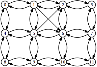
| 0 | 1 | 2 | 3 | 4 | 5 | 6 | 7 | 8 | 9 | 10 | 11 | |
|---|---|---|---|---|---|---|---|---|---|---|---|---|
| 0 | 0 | 1 | 0 | 0 | 1 | 0 | 0 | 0 | 0 | 0 | 0 | 0 |
| 1 | 1 | 0 | 1 | 0 | 0 | 1 | 1 | 0 | 0 | 0 | 0 | 0 |
| 2 | 1 | 0 | 0 | 1 | 0 | 0 | 1 | 0 | 0 | 0 | 0 | 0 |
| 3 | 0 | 0 | 1 | 0 | 0 | 0 | 0 | 1 | 0 | 0 | 0 | 0 |
| 4 | 1 | 0 | 0 | 0 | 0 | 1 | 0 | 0 | 1 | 0 | 0 | 0 |
| 5 | 0 | 1 | 1 | 0 | 1 | 0 | 1 | 0 | 0 | 1 | 0 | 0 |
| 6 | 0 | 0 | 1 | 0 | 0 | 1 | 0 | 1 | 0 | 0 | 1 | 0 |
| 7 | 0 | 0 | 0 | 1 | 0 | 0 | 1 | 0 | 0 | 0 | 0 | 1 |
| 8 | 0 | 0 | 0 | 0 | 1 | 0 | 0 | 0 | 0 | 1 | 0 | 0 |
| 9 | 0 | 0 | 0 | 0 | 0 | 1 | 0 | 0 | 1 | 0 | 1 | 0 |
| 10 | 0 | 0 | 0 | 0 | 0 | 0 | 1 | 0 | 0 | 1 | 0 | 1 |
| 11 | 0 | 0 | 0 | 0 | 0 | 0 | 0 | 1 | 0 | 0 | 1 | 0 |
Where the adjacency matrix performs poorly is with the \(\mathtt{outEdges(i)}\) and \(\mathtt{inEdges(i)}\) operations. To implement these, we must scan all \(\mathtt{n}\) entries in the corresponding row or column of \(\mathtt{a}\) and gather up all the indices, \(\mathtt{j}\), where \(\mathtt{a[i][j]}\), respectively \(\mathtt{a[j][i]}\), is true.
    List<Integer> outEdges(int i) {
        List<Integer> edges = new ArrayList<Integer>();
        for (int j = 0; j < n; j++)
            if (a[i][j]) edges.add(j);
        return edges;
    }
    List<Integer> inEdges(int i) {
        List<Integer> edges = new ArrayList<Integer>();
        for (int j = 0; j < n; j++)
            if (a[j][i]) edges.add(j);
        return edges;
    }
These operations clearly take \(O(\mathtt{n})\) time per operation.
Another drawback of the adjacency matrix representation is that it is large. It stores an \(\mathtt{n}\times \mathtt{n}\) boolean matrix, so it requires at least \(\mathtt{n}^2\) bits of memory. The implementation here uses a matrix of \(\mathtt{boolean}\) values so it actually uses on the order of \(\mathtt{n}^2\) bytes of memory. A more careful implementation, which packs \(\mathtt{w}\) boolean values into each word of memory, could reduce this space usage to \(O(\mathtt{n}^2/\mathtt{w})\) words of memory.
Theorem \(\PageIndex{1}\)
The AdjacencyMatrix data structure implements the Graph interface. An AdjacencyMatrix supports the operations
- \(\mathtt{addEdge(i,j)}\), \(\mathtt{removeEdge(i,j)}\), and \(\mathtt{hasEdge(i,j)}\) in constant time per operation; and
- \(\mathtt{inEdges(i)}\), and \(\mathtt{outEdges(i)}\) in \(O(\mathtt{n})\) time per operation.
The space used by an AdjacencyMatrix is \(O(\mathtt{n}^2)\).
Despite its high memory requirements and poor performance of the \(\mathtt{inEdges(i)}\) and \(\mathtt{outEdges(i)}\) operations, an AdjacencyMatrix can still be useful for some applications. In particular, when the graph \(G\) is dense, i.e., it has close to \(\mathtt{n}^2\) edges, then a memory usage of \(\mathtt{n}^2\) may be acceptable.
The AdjacencyMatrix data structure is also commonly used because algebraic operations on the matrix \(\mathtt{a}\) can be used to efficiently compute properties of the graph \(G\). This is a topic for a course on algorithms, but we point out one such property here: If we treat the entries of \(\mathtt{a}\) as integers (1 for \(\mathtt{true}\) and 0 for \(\mathtt{false}\)) and multiply \(\mathtt{a}\) by itself using matrix multiplication then we get the matrix \(\mathtt{a}^2\). Recall, from the definition of matrix multiplication, that
\[\mathtt{a^2[i][j]} = \sum_{k=0}^{\mathtt{n}-1} \mathtt{a[i][k]}\cdot \mathtt{a[k][j]} \enspace .\nonumber\]
Interpreting this sum in terms of the graph \(G\), this formula counts the number of vertices, \(\mathtt{k}\), such that \(G\) contains both edges \(\mathtt{(i,k)}\) and \(\mathtt{(k,j)}\). That is, it counts the number of paths from \(\mathtt{i}\) to \(\mathtt{j}\) (through intermediate vertices, \(\mathtt{k}\)) whose length is exactly two. This observation is the foundation of an algorithm that computes the shortest paths between all pairs of vertices in \(G\) using only \(O(\log \mathtt{n})\) matrix multiplications.