8.6: Machine Code and Branching

In order to understand how branch addresses are calculated, it is first necessary to understand how data is stored, or more specifically, how data is aligned in memory when it is stored. When loading data from memory, the data is passed from the memory to a register value as 32 bits. However the 32 bits in memory are not any 32 bits. Remember that the ARM computer is byte addressable, so only groups of 8 bits (or a byte) can be used to specify an address.

There is another constraint on the data being passed from memory to a register, that is that the data passed from memory to a register must be word aligned. For the 32-bit ARM CPU, word alignment means that memory is grouped into collections of 4-byte words, and the transfers occur on words. Thus the memory at addresses 0x0, 0x4, 0x8, 0xc, 0x10, etc., can be transferred from memory to a register. Addresses that are smaller in size than a word (e.g. a byte using ldrb or ldrsb, or half word using ldrh or ldrsh) will still access a byte, but will fixup the value so that it keeps memory correct.

Note that alignment is easy to check since all addresses are byte aligned, the address for a half word align on an even addresses, word align on an addresses divisible by 4, and double word addresses align on an address divisible by 8. Therefore only the last nybble (4 bits) of the address need to be checked to see if the address is aligned. For example, if the last nybble is 0x [0, 2, 4, 6, 8, a, c, or e] or binary 0b...0, it is half-word aligned. If the last nybble is 0x[0, 4, 8, or c] or 0b..00, it is word aligned, and if it is 0x[0,8], or 0b.000, it is double word aligned.

Note that all instructions for the ARM 32 bit architecture are word aligned. This means that the last two bits of all instructions are 0b00. This will have implications in the next section on calculating a branch address.

8.6.1 Endianness

Since data storage is being discussed, this is a good place to discuss one of the religious wars that break out now and again in all sciences. In this case, the idea of Big-Endian and LittleEndian. The terms, borrowed them from Jonathan Swift who in Gulliver's Travels used them to describe the opposing positions of two factions in the nation of Lilliput. One side broke their boiled eggs at the big end, rebelled against the king, who demanded that his subjects break their eggs at the little end. The story illustrates useless wars about unimportant topics.

The idea of endianness is another such unimportant discussion. First realize that all bits in a byte are numbered in the same order. The order is high order to low order byte, as shown in the following diagram:

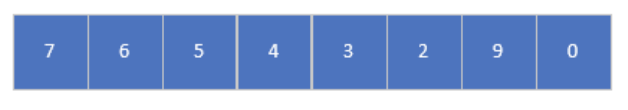
This means that the binary string 0b001 1100 = 0x1c = \(28_{10}\). Note that the byte might not be a number, but could be a character, part of an address, or part of an instruction. The number represented here is just to point out the order of the bits in a bytes.

The question is what ordering to use to present bytes. For example, in a Big-Endian 4 bytes can be represented in such a way as to make the strings make sense, e.g

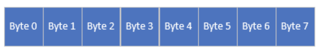
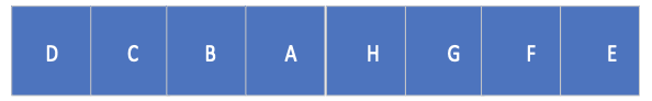
This allows the string “ABCDEFGH” to appear as follows when it is viewed in memory .

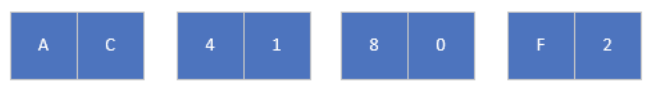
However, if you want to see the number 2,889,974,002 = 0xAC4180F2, it would look as follows in memory (note that each byte is 2 hex digits, so this number is 4 bytes).

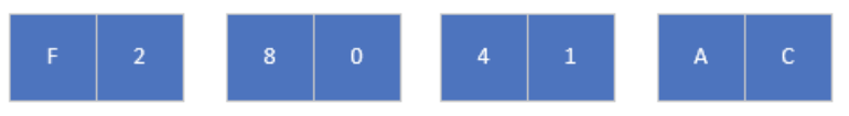
This strange representation for the numeric value can be fixed by using Little-Endian format, or representing bytes as follows:

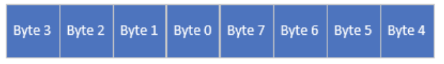
This gives the correct result for numeric values:

But the string of characters is strange.

So which format is correct, Big-Endian or Little-Endian? This is really a religious argument, where both sides believe firmly they are correct, but neither side is right or wrong. The argument is inane argument because to the computer architecture it simply doesn’t matter. It only matters to someone trying to read the memory, and even then the tools to look at the memory can presented as the user wants to see it.

The ARM architecture will support either format, so the choice is really arbitrary. If you work in an environment where most of the computers are Big-Endian, you would probably decide to use Big-Endian. The same with Little-Endian.

The real issue occurs when transferring data between computers. When doing data transfer, most languages provide functions that allow programs to format data into a network format. This is an agreed upon standard that allows data to be transferred between computer with different data storage types. Otherwise, the issue of Endianness can, and should, to left to computer bigots and care.

8.6.2 Calculating a branch address

The PC contains the address of the instruction to execute, so branching in a CPU implies that the PC is changed to a new value. The question is how to calculate the new value to use for the PC. To do this, two types of addressing will be introduced, PC relative addressing and absolute addressing.

Of the two types of addressing, the concept of absolute addressing is easiest to understand. A absolute address is an absolute address in memory. This is illustrated in the following diagram, where the address of memory of the instruction to execute is 0x35fc. To branch to this address all that would be necessary is that the PC be set to this value (e.g. MOV pc, #0x35fc), and the code would begin executing at the new address. Absolute addressing is easy to understand, but is somewhat difficult to implement. When compiling and assembling a program, the absolute addresses of the machine instructions is not yet know. Absolute instruction address at assigned when the program is linked, and thus the calculation of the addresses must be deferred until link time. In addition, the addresses are then fixed, and the code cannot be moved after the absolute address is assigned. This make using absolute addressing problematic, and it is generally only used or functions and a few variables that are created and/or used in a separate file from the one being assembled or compiled.

If absolute addressing is not used, then how are addresses calculate? The answer is that when executing a program, the absolute address of the PC is known. If the distance from the PC to another instruction is also known, the address of the instruction to branch to can be calculated by adding that distance to the PC, and the absolute address of that statement can be calculated. This is known as PC relative addressing.

In PC relative addressing, the assembler or compiler can calculate the distance from any statement to any other statement in the same file. Consider the following example. In this example, the “B label_1” statement intends to branch to label_1. The branch instruction passes the distance of the branch statement to label_1 to the CPU, and the CPU calculates and branches to that instruction.

Before showing how to calculate a branch, there are important considerations for calculating branches. First, because the instructions are all 4 bytes big, each instruction is 4 bytes from the previous instruction, so you would think that the each instruction would add 4 to the distance value to branch. However, because the instructions are word aligned, the final two zeros are dropped from the distance value. This means that the distance used in the branch instruction can be obtained by counting the number of instructions between the branch statement and the instruction to be branched to. Note that this trick works, but is not representative of what is really happening.

Second, when the branch is actually calculated, the value in the PC is the PC of the branch instruction plus 8. So when executing the branch, you should start counting at the instruction two ahead of the current branch instruction when calculating the branch distance. Thus in this example, the PC at the “B label_1” statement is 0x35e8, but the distance used in the branch statement is 3 (0x35e8 + 8 + 3*4 = 0x35fc).

Branching can be in a forward or reverse direction. So the “B label_2” in the previous code fragment branches backward in the program, and the distance for the branch is negative.

The same address calculations are done on the memory data in the program. Note that in this case address of var_1 is ??? from the PC, and var_2 is -4. Why var_2 is -4, even though it occurs after the statement which uses the variable, is left as an exercise at the end of the chapter.