5.1: Turing Machines
- Page ID
- 6736
\( \newcommand{\vecs}[1]{\overset { \scriptstyle \rightharpoonup} {\mathbf{#1}} } \)
\( \newcommand{\vecd}[1]{\overset{-\!-\!\rightharpoonup}{\vphantom{a}\smash {#1}}} \)
\( \newcommand{\id}{\mathrm{id}}\) \( \newcommand{\Span}{\mathrm{span}}\)
( \newcommand{\kernel}{\mathrm{null}\,}\) \( \newcommand{\range}{\mathrm{range}\,}\)
\( \newcommand{\RealPart}{\mathrm{Re}}\) \( \newcommand{\ImaginaryPart}{\mathrm{Im}}\)
\( \newcommand{\Argument}{\mathrm{Arg}}\) \( \newcommand{\norm}[1]{\| #1 \|}\)
\( \newcommand{\inner}[2]{\langle #1, #2 \rangle}\)
\( \newcommand{\Span}{\mathrm{span}}\)
\( \newcommand{\id}{\mathrm{id}}\)
\( \newcommand{\Span}{\mathrm{span}}\)
\( \newcommand{\kernel}{\mathrm{null}\,}\)
\( \newcommand{\range}{\mathrm{range}\,}\)
\( \newcommand{\RealPart}{\mathrm{Re}}\)
\( \newcommand{\ImaginaryPart}{\mathrm{Im}}\)
\( \newcommand{\Argument}{\mathrm{Arg}}\)
\( \newcommand{\norm}[1]{\| #1 \|}\)
\( \newcommand{\inner}[2]{\langle #1, #2 \rangle}\)
\( \newcommand{\Span}{\mathrm{span}}\) \( \newcommand{\AA}{\unicode[.8,0]{x212B}}\)
\( \newcommand{\vectorA}[1]{\vec{#1}} % arrow\)
\( \newcommand{\vectorAt}[1]{\vec{\text{#1}}} % arrow\)
\( \newcommand{\vectorB}[1]{\overset { \scriptstyle \rightharpoonup} {\mathbf{#1}} } \)
\( \newcommand{\vectorC}[1]{\textbf{#1}} \)
\( \newcommand{\vectorD}[1]{\overrightarrow{#1}} \)
\( \newcommand{\vectorDt}[1]{\overrightarrow{\text{#1}}} \)
\( \newcommand{\vectE}[1]{\overset{-\!-\!\rightharpoonup}{\vphantom{a}\smash{\mathbf {#1}}}} \)
\( \newcommand{\vecs}[1]{\overset { \scriptstyle \rightharpoonup} {\mathbf{#1}} } \)
\( \newcommand{\vecd}[1]{\overset{-\!-\!\rightharpoonup}{\vphantom{a}\smash {#1}}} \)
\(\newcommand{\avec}{\mathbf a}\) \(\newcommand{\bvec}{\mathbf b}\) \(\newcommand{\cvec}{\mathbf c}\) \(\newcommand{\dvec}{\mathbf d}\) \(\newcommand{\dtil}{\widetilde{\mathbf d}}\) \(\newcommand{\evec}{\mathbf e}\) \(\newcommand{\fvec}{\mathbf f}\) \(\newcommand{\nvec}{\mathbf n}\) \(\newcommand{\pvec}{\mathbf p}\) \(\newcommand{\qvec}{\mathbf q}\) \(\newcommand{\svec}{\mathbf s}\) \(\newcommand{\tvec}{\mathbf t}\) \(\newcommand{\uvec}{\mathbf u}\) \(\newcommand{\vvec}{\mathbf v}\) \(\newcommand{\wvec}{\mathbf w}\) \(\newcommand{\xvec}{\mathbf x}\) \(\newcommand{\yvec}{\mathbf y}\) \(\newcommand{\zvec}{\mathbf z}\) \(\newcommand{\rvec}{\mathbf r}\) \(\newcommand{\mvec}{\mathbf m}\) \(\newcommand{\zerovec}{\mathbf 0}\) \(\newcommand{\onevec}{\mathbf 1}\) \(\newcommand{\real}{\mathbb R}\) \(\newcommand{\twovec}[2]{\left[\begin{array}{r}#1 \\ #2 \end{array}\right]}\) \(\newcommand{\ctwovec}[2]{\left[\begin{array}{c}#1 \\ #2 \end{array}\right]}\) \(\newcommand{\threevec}[3]{\left[\begin{array}{r}#1 \\ #2 \\ #3 \end{array}\right]}\) \(\newcommand{\cthreevec}[3]{\left[\begin{array}{c}#1 \\ #2 \\ #3 \end{array}\right]}\) \(\newcommand{\fourvec}[4]{\left[\begin{array}{r}#1 \\ #2 \\ #3 \\ #4 \end{array}\right]}\) \(\newcommand{\cfourvec}[4]{\left[\begin{array}{c}#1 \\ #2 \\ #3 \\ #4 \end{array}\right]}\) \(\newcommand{\fivevec}[5]{\left[\begin{array}{r}#1 \\ #2 \\ #3 \\ #4 \\ #5 \\ \end{array}\right]}\) \(\newcommand{\cfivevec}[5]{\left[\begin{array}{c}#1 \\ #2 \\ #3 \\ #4 \\ #5 \\ \end{array}\right]}\) \(\newcommand{\mattwo}[4]{\left[\begin{array}{rr}#1 \amp #2 \\ #3 \amp #4 \\ \end{array}\right]}\) \(\newcommand{\laspan}[1]{\text{Span}\{#1\}}\) \(\newcommand{\bcal}{\cal B}\) \(\newcommand{\ccal}{\cal C}\) \(\newcommand{\scal}{\cal S}\) \(\newcommand{\wcal}{\cal W}\) \(\newcommand{\ecal}{\cal E}\) \(\newcommand{\coords}[2]{\left\{#1\right\}_{#2}}\) \(\newcommand{\gray}[1]{\color{gray}{#1}}\) \(\newcommand{\lgray}[1]{\color{lightgray}{#1}}\) \(\newcommand{\rank}{\operatorname{rank}}\) \(\newcommand{\row}{\text{Row}}\) \(\newcommand{\col}{\text{Col}}\) \(\renewcommand{\row}{\text{Row}}\) \(\newcommand{\nul}{\text{Nul}}\) \(\newcommand{\var}{\text{Var}}\) \(\newcommand{\corr}{\text{corr}}\) \(\newcommand{\len}[1]{\left|#1\right|}\) \(\newcommand{\bbar}{\overline{\bvec}}\) \(\newcommand{\bhat}{\widehat{\bvec}}\) \(\newcommand{\bperp}{\bvec^\perp}\) \(\newcommand{\xhat}{\widehat{\xvec}}\) \(\newcommand{\vhat}{\widehat{\vvec}}\) \(\newcommand{\uhat}{\widehat{\uvec}}\) \(\newcommand{\what}{\widehat{\wvec}}\) \(\newcommand{\Sighat}{\widehat{\Sigma}}\) \(\newcommand{\lt}{<}\) \(\newcommand{\gt}{>}\) \(\newcommand{\amp}{&}\) \(\definecolor{fillinmathshade}{gray}{0.9}\)Historically, the theoretical study of computing began before computers ex- isted. One of the early models of computation was developed in the 1930s by the British mathematician, Alan Turing, who was interested in study- ing the theoretical abilities and limitations of computation. His model for computation is a very simple abstract computing machine which has come to be known as a Turing machine. While Turing machines are not appli- cable in the same way that regular expressions, finite-state automata, and grammars are applicable, their use as a fundamental model for computation means that every computer scientist should be familiar with them, at least in a general way.
A Turing machine is really not much more complicated than a finitestateautomatonorapushdownautomaton.1 Like a FSA, a Turing machine has a finite number of possible states, and it changes from state to state as it computes. However, a Turing machine also has an infinitely long tape that it can use for input and output. The tape extends to infinity in both directions. The tape is divided into cells, which are in one-to-one correspondence with the integers, Z. Each cell can either be blank or it can hold a symbol from a specified alphabet. The Turing machine can move back and forth along this tape, reading and writing symbols and changing state. It can read only one cell at a time, and possibly write a new value in that cell. After doing this, it can change state and it can move by one cell either to the left or to the right. This is how the Turing machine computes. To use a Turing machine, you would write some input on its tape, start the machine, and let it compute until it halts. Whatever is written on the tape at that time is the output of the computation.
Although the tape is infinite, only a finite number of cells can be non- blank at any given time. If you don’t like the idea of an infinite tape, you can think of a finite tape that can be extended to an arbitrarily large size as the Turing machine computes: If the Turing machine gets to either end of the tape, it will pause and wait politely until you add a new section of tape. In other words, it’s not important that the Turing machine have an infinite amount of memory, only that it can use as much memory as it needs for a given computation, up to any arbitrarily large size. In this way, a Turing machine is like a computer that can ask you to buy it a new disk drive whenever it needs more storage space to continue a computation.2
A given Turing machine has a fixed, finite set of states. One of these states is designated as the start state. This is the state in which the Turing machine begins a computation. Another special state is the halt state. The Turing machine’s computation ends when it enters its halt state. It is possible that a computation might never end because the machine never enters the halt state. This is analogous to an infinite loop in a computer program.
At each step in its computation, the Turing machine reads the contents of the tape cell where it is located. Depending on its state and the symbol that it reads, the machine writes a symbol (possibly the same symbol) to the cell, moves one cell either to the left or to the right, and (possibly) changes its state. The output symbol, direction of motion, and new state are determined by the current state and the input symbol. Note that either the input symbol, the output symbol, or both, can be blank. A Turing machine has a fixed set of rules that tell it how to compute. Each rule specifies the output symbol, direction of motion, and new state for some combination of current state and input symbol. The machine has a rule for every possible combination of current state and input symbol, except that there are no rules for what happens if the current state is the halt state. Of course, once the machine enters the halt state, its computation is complete and the machine simply stops.
I will use the character # to represent a blank in a way that makes it visible. I will always use h to represent the halt state. I will indicate the directions, left and right, with L and R, so that {L,R} is the set of possible directions of motion. With these conventions, we can give the formal definition of a Turing machine as follows:
Definition 5.1.
A Turing machine is a 4-tuple \(\left(Q, \Lambda, q_{0}, \delta\right)\), where
- Q is a finite set of states, including the halt state, h.
- Λ is an alphabet which includes the blank symbol, #.
- \(q_{0} \in Q\) is the start state.
- \(\delta :(Q \backslash\{h\}) \times \Lambda \rightarrow \Lambda \times\{L, R\} \times Q\) is the transition function. The fact that \(\delta(q, \sigma)=(\tau, d, r)\) means that when the Turing machine is in state q and reads the symbol σ, it writes the symbol τ, moves one cell in the direction d, and enters state r.
Even though this is the formal definition, it’s easier to work with a tran- sition diagram representation of Turing machines. The transition diagram for a Turing machine is similar to the transition diagram for a DFA. How- ever, there are no “accepting” states (only a halt state). Furthermore, there must be a way to specify the output symbol and the direction of motion for each step of the computation. We do this by labeling arrows with notations of the form \((\sigma, \tau, L)\) and \((\sigma, \tau, R),\) where \(\sigma\) and \(\tau\) are symbols in the Turing machine’s alphabet. For example,
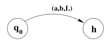
indicates that when the machine is in state \(q_{0}\) and reads an a, it writes ab, moves left, and enters state h.
Here, for example, is a transition diagram for a simple Turing machine that moves to the right, changing a’s to b’s and vice versa, until it finds ac. It leaves blanks (#’s) unchanged. When and if the machine encounters ac, it moves to the left and halts:
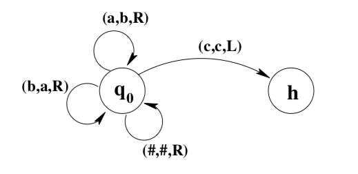
To simplify the diagrams, I will leave out any transitions that are not relevant to the computation that I want the machine to perform. You can assume that the action for any omitted transition is to write the same symbol that was read, move right, and halt.
For example, shown below is a transition diagram for a Turing machine that makes a copy of a string of a’s and b’s. To use this machine, you would write a string of a’s and b’s on its tape, place the machine on the first character of the string, and start the machine in its start state, q0. When the machine halts, there will be two copies of the string on the tape, separated by a blank. The machine will be positioned on the first character of the leftmost copy of the string. Note that this machine uses c’s and d’s in addition to a’s and b’s. While it is copying the input string, it temporarily changes the a’s and b’s that it has copied to c’s and d’s, respectively. In this way it can keep track of which characters it has already copied. After the string has been copied, the machine changes the c’s and d’s back to a’s and b’s before halting.
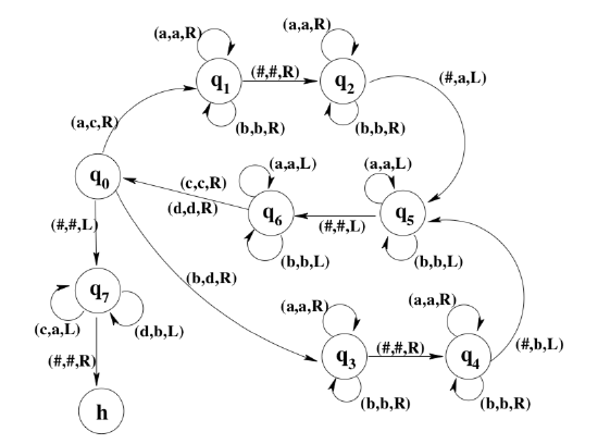
In this machine, state q0 checks whether the next character is an a, a \(b,\) or a \(\#\) (indicating the end of the string). States \(q_{1}\) and \(q_{2}\) add an \(a\) to the end of the new string, and states \(q_{3}\) and \(q_{4}\) do the same thing with a b. States \(q_{5}\) and \(q_{6}\) return the machine to the next character in the input string. When the end of the input string is reached, state \(q_{7}\) will move the machine back to the start of the input string, changing c’s and d’s back toa’s and b’s as it goes. Finally, when the machine hits the # that precedes the input string, it moves to the right and halts. This leave it back at the first character of the input string. It would be a good idea to work through the execution of this machine for a few sample input strings. You should also check that it works even for an input string of length zero.
Our primary interest in Turing machines is as language processors. Sup- pose that w is a string over an alphabet Σ. We will assume that Σ does not contain the blank symbol. We can use w as input to a Turing machine \(M=\left(Q, \Lambda, q_{0}, \delta\right)\) provided that \(\Sigma \subseteq \Lambda .\) To use \(w\) as input for \(M\) we will write w on M’s tape and assume that the remainder of the tape is blank. We place the machine on the cell containing the first character of the string, except that if \(w=\varepsilon\) then we simply place the machine on a completely blank tape. Then we start the machine in its initial state, \(q_{0}\) and see what computation it performs. We refer to this setup as “runningM with input w.”
When M is run with input w, it is possible that it will just keep running forever without halting. In that case, it doesn’t make sense to ask about the output of the computation. Suppose however that M does halt on inputw. Suppose, furthermore, that when M halts, its tape is blank except for a string x of non-blank symbols, and that the machine is located on the first character of x. In this case, we will say that “M halts with output x.” In addition, if M halts with an entirely blank tape, we say that “M halts with output ε.” Note that when we run M with input w, one of three things can happen: (1) M might halt with some string as output; (1) M might fail to halt; or (3) M might halt in some configuration that doesn’t count as outputting any string.
The fact that a Turing machine can produce an output value allows us for the first time to deal with computation of functions. A function \(f : A \rightarrow B\) takes an input value in the set \(A\) and produces an output value in the set B. If the sets are sets of strings, we can now ask whether the values of the function can be computed by a Turing machine. That is, is there a Turing machine M such that, given any string w in the domain off as input, M will compute as its output the string f(w). If this is that case, then we say that f is a Turing-computable function.
Definition 5.2.
Suppose that \(\Sigma\) and \(\Gamma\) are alphabets that do not contain \(\#\) and that \(f\) is a function from \(\Sigma^{*}\) to \(\Gamma^{*} .\) We say that \(f\) is Turing-computable if there is a Turing machine \(M=\left(Q, \Lambda, q_{0}, \delta\right)\) such that \(\Sigma \subseteq \Lambda\) and \(\Gamma \subseteq \Lambda\) and for each string \(w \in \Sigma^{*},\) when \(M\) is run with input w, it halts with output f(w). In this case, we say that M computes the function f.
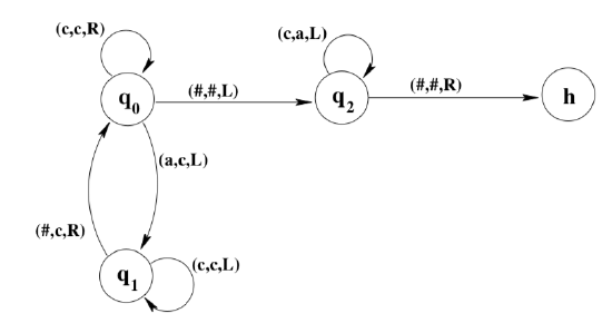
For example, let \(\Sigma=\{a\}\) and define \(f : \Sigma^{*} \rightarrow \Sigma^{*}\) by \(f\left(a^{n}\right)=a^{2 n},\) for \(n \in \mathbb{N} .\) Then \(f\) is Turing-computable since it is computed by this Turing machine:
We can also use Turing machines to define “computable languages.” There are actually two different notions of Turing-computability for lan- guages. One is based on the idea of Turing-computability for functions. Suppose that \(\Sigma\) is an alphabet and that \(L \subseteq \Sigma^{*} .\) The characteristic function of \(L\) is the function \(\chi_{L} : \Sigma^{*} \rightarrow\{0,1\}\) defined by the fact that \(\chi_{L}(w)=1\) if \(w \in L\) and \(\chi_{L}(w)=0\) if \(w \notin L .\) Note that given the function \(\chi_{L}, L\) can be obtained as the set \(L=\left\{w \in \Sigma^{*} | \chi_{L}(w)=1\right\} .\) Given a language \(L,\) we can ask whether the corresponding function \(\chi_{L}\) is Turing-computable. If so, then we can use a Turing machine to decide whether or not a given string w is in L. Just run the machine with input w. It will halt with output \(\chi_{L}(w) .\) (That is, it will halt and when it does so, the tape will be blank except for a 0 or a 1, and the machine will be positioned on the 0 or \(1 . )\) If the machine halts with output \(1,\) then \(w \in L .\) If the machine halts with output \(0,\) then \(w \notin L\).
Definition 5.3.
Let \(\Sigma\) be an alphabet that does not contain \(\#\) and let \(L\) be a language over \(\Sigma .\) We say that \(L\) is Turing-decidable if there is a Turing machine \(M=\left(Q, \Lambda, q_{0}, \delta\right)\) such that \(\Sigma \subseteq \Lambda,\{0,1\} \subseteq \Lambda,\) and for each \(w \in \Sigma^{*},\) when \(M\) is run with input \(w,\) it halts with output \(\chi_{L}(w)\) (That is, it halts with output 0 or \(1,\) and the output is 0 if \(w \notin L\) and is 1 if \(w \in L .\) ) In this case, we say that \(M\) decides the language \(L\)
The second notion of computability for languages is based on the inter- esting fact that it is possible for a Turing machine to run forever, without ever halting. Whenever we run a Turing machine M with input w, we can ask the question, will M ever halt or will it run forever? If M halts on inputw, we will say that M “accepts” w. We can then look at all the strings over a given alphabet that are accepted by a given Turing machine. This leads to the notion of Turing-acceptable languages.
Definition 5.4.
Let \(\Sigma\) be an alphabet that does not contain \(\#,\) and let \(L\) be a language over \(\Sigma .\) We say that \(L\) is Turing-acceptable if there is a Turing machine \(M=\left(Q, \Lambda, q_{0}, \delta\right)\) such that \(\Sigma \subseteq \Lambda,\) and for each \(w \in \Sigma^{*}\) \(M\) halts on input \(w\) if and only if \(w \in L .\) In this case, we say that \(M\) accepts the language L.
It should be clear that any Turing-decidable language is Turing-acceptable. In fact, if \(L\) is a language over an alphabet \(\Sigma,\) and if \(M\) is a Turing machine that decides L, then it is easy to modify M to produce a Turing machine that accepts L. At the point where M enters the halt state with output 0, the new machine should enter a new state in which it simply moves to the right forever, without ever halting. Given an input \(w \in \Sigma^{*},\) the modified machine will halt if and only if M halts with output 1, that is, if and only if \(w \in L\).
Exercises
- Let \(\Sigma=\{a\} .\) Draw a transition diagram for a Turing machine that computes the function \(f : \Sigma^{*} \rightarrow \Sigma^{*}\) where \(f\left(a^{n}\right)=a^{3 n},\) for \(n \in \mathbb{N} .\) Draw a transition diagram for a Turing machine that computes the function \(f : \Sigma^{*} \rightarrow \Sigma^{*}\) where \(f\left(a^{n}\right)=a^{3 n+1},\) for \(n \in \mathbb{N}\).
- Let \(\Sigma=\{a, b\} .\) Draw a transition diagram for a Turing machine that computes the function \(f : \Sigma^{*} \rightarrow \Sigma^{*}\) where \(f(w)=w^{R}\).
3.Suppose that \(\Sigma, \Gamma,\) and \(\Xi\) are alphabets and that \(f : \Sigma^{*} \rightarrow \Gamma^{*}\) and \(g : \Gamma^{*} \rightarrow \Xi^{*}\) are Turing-computable functions. Show that \(g \circ f\) is Turing-computable.
- We have defined computability for functions \(f : \Sigma^{*} \rightarrow \Gamma^{*},\) where \(\Sigma\) and \(\Gamma\) are alphabets. How could Turing machines be used to define computable functions from \(\mathbb{N}\) to \(\mathbb{N} ?\) (Hint: Consider the alphabet \(\Sigma=\{a\} . )\)
- Let \(\Sigma\) be an alphabet and let \(L\) be a language over \(\Sigma .\) Show that \(L\) is Turing-decidable if and only if its complement, \(\overline{L},\) is Turing-decidable.
- Draw a transition diagram for a Turing machine which decides the language \(\left\{a^{n} b^{n} | n \in \mathbb{N}\right\} .\) (Hint: Change the \(a^{\prime}\) s and \(b\) 's to \(\$^{\prime} \mathrm{s}\) in pairs.) Explain in general terms how to make a Turing machine that decides the language \(\left\{a^{n} b^{n} c^{n} | n \in \mathbb{N}\right\}\).
- Draw a transition diagram for a Turing machine which decides the language \(\left\{a^{n} b^{m} | n>0 \text { and } m \text { is a multiple of } n\right\} .\) (Hint: Erase \(n b^{\prime}\) s at a time.)
- Based on your answer to the previous problem and the copying machine presented in this section, describe in general terms how you would build a Turing machine to decide the language \(\left\{a^{p} | p \text { is a prime number }\right\}\).
- Let \(g :\{a\}^{*} \rightarrow\{0,1\}^{*}\) be the function such that for each \(n \in \mathbb{N}, g\left(a^{n}\right)\) is the representation of n as a binary number. Draw a transition diagram for a Turing machine that computes g.


