12.2: Definitions of Planar Graphs

We took the idea of a planar drawing for granted in the previous section, but if we’re going to prove things about planar graphs, we better have precise definitions.

Definition \(\PageIndex{1}\)

A drawing of a graph assigns to each node a distinct point in the plane and assigns to each edge a smooth curve in the plane whose endpoints correspond to the nodes incident to the edge. The drawing is planar if none of the curves cross themselves or other curves, namely, the only points that appear more than once on any of the curves are the node points. A graph is planar when it has a planar drawing.

Definition 12.2.1 is precise but depends on further concepts: “smooth planar curves” and “points appearing more than once” on them. We haven’t defined these concepts —we just showed the simple picture in Figure 12.4 and hoped you would get the idea.

Pictures can be a great way to get a new idea across, but it is generally not a good idea to use a picture to replace precise mathematics. Relying solely on pictures can sometimes lead to disaster —or to bogus proofs, anyway. There is a long history of bogus proofs about planar graphs based on misleading pictures.

The bad news is that to prove things about planar graphs using the planar drawings of Definition 12.2.1, we’d have to take a chapter-long excursion into continuous mathematics just to develop the needed concepts from plane geometry and point-set topology. The good news is that there is another way to define planar graphs that uses only discrete mathematics. In particular, we can define planar graphs as a recursive data type. In order to understand how it works, we first need to understand the concept of a face in a planar drawing.

Faces

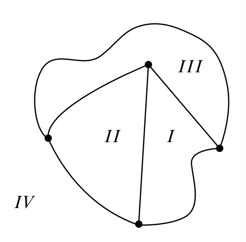
The curves in a planar drawing divide up the plane into connected regions called the continuous faces¹ of the drawing. For example, the drawing in Figure 12.5 has four continuous faces. Face IV, which extends off to infinity in all directions, is called the outside face.

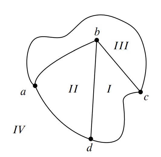
The vertices along the boundary of each continuous face in Figure 12.5 form a cycle. For example, labeling the vertices as in Figure 12.6, the cycles for each of the face boundaries can be described by the vertex sequences

\[\label{12.2.1.} abca \quad abda \quad bcdb \quad acda.\]

These four cycles correspond nicely to the four continuous faces in Figure 12.6 — so nicely, in fact, that we can identify each of the faces in Figure 12.6 by its cycle. For example, the cycle \(abca\) identifies face III. The cycles in list \(\ref{12.2.1.}\) are called the discrete faces of the graph in Figure 12.6. We use the term “discrete” since cycles in a graph are a discrete data type —as opposed to a region in the plane, which is a continuous data type.

Figure 12.5 A planar drawing with four continuous faces.

Figure 12.6 The drawing with labeled vertices.

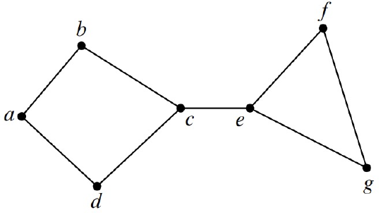
Unfortunately, continuous faces in planar drawings are not always bounded by cycles in the graph —things can get a little more complicated. For example, the planar drawing in Figure 12.7 has what we will call a bridge, namely, a cut edge \(\langle c - e \rangle\). The sequence of vertices along the boundary of the outer region of the drawing is

\[\nonumber abcefgecda.\]

This sequence defines a closed walk, but does not define a cycle since the walk has two occurrences of the bridge \(\langle c - e \rangle\) and each of its endpoints.

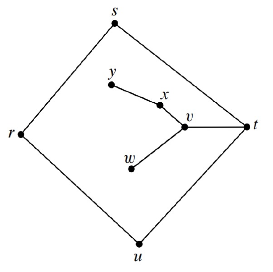
The planar drawing in Figure 12.8 illustrates another complication. This drawing has what we will call a dongle, namely, the nodes \(v, x, y,\) and \(w\), and the edges incident to them. The sequence of vertices along the boundary of the inner region is

\[\nonumber rstvxyxvwvtur.\]

This sequence defines a closed walk, but once again does not define a cycle because it has two occurrences of every edge of the dongle —once “coming” and once “going.”

It turns out that bridges and dongles are the only complications, at least for connected graphs. In particular, every continuous face in a planar drawing corresponds to a closed walk in the graph. These closed walks will be called the discrete faces of the drawing, and we’ll define them next.

Figure 12.7 A planar drawing with a bridge.

Figure 12.8 A planar drawing with a dongle.

Recursive Definition for Planar Embeddings

The association between the continuous faces of a planar drawing and closed walks provides the discrete data type we can use instead of continuous drawings. We’ll define a planar embedding of connected graph to be the set of closed walks that are its face boundaries. Since all we care about in a graph are the connections between vertices —not what a drawing of the graph actually looks like —planar embeddings are exactly what we need.

The question is how to define planar embeddings without appealing to continuous drawings. There is a simple way to do this based on the idea that any continuous drawing can drawn step by step:

• either draw a new point somewhere in the plane to represent a vertex,
• or draw a curve between two vertex points that have already been laid down, making sure the new curve doesn’t cross any of the previously drawn curves.

A new curve won’t cross any other curves precisely when it stays within one of the continuous faces. Alternatively, a new curve won’t have to cross any other curves if it can go between the outer faces of two different drawings. So to be sure it’s ok to draw a new curve, we just need to check that its endpoints are on the boundary of the same face, or that its endpoints are on the outer faces of different drawings. Of course drawing the new curve changes the faces slightly, so the face boundaries will have to be updated once the new curve is drawn. This is the idea behind the following recursive definition.

Definition \(\PageIndex{2}\)

A planar embedding of a connected graph consists of a nonempty set of closed walks of the graph called the discrete faces of the embedding. Planar embeddings are defined recursively as follows:

Base case: If G is a graph consisting of a single vertex, \(v\), then a planar embedding of \(G\) has one discrete face, namely, the length zero closed walk, \(v\).

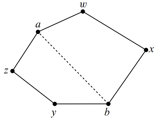
Constructor case (split a face): Suppose \(G\) is a connected graph with a planar embedding, and suppose \(a\) and \(b\) are distinct, nonadjacent vertices of \(G\) that occur in some discrete face, \(\gamma\), of the planar embedding. That is, \(\gamma\) is a closed walk of the form

\[\nonumber \gamma = \alpha \hat{} \beta\]

where \(\alpha\) is a walk from \(a\) to \(b\) and \(\beta\) is a walk from \(b\) to \(a\). Then the graph obtained by adding the edge \(\langle a - b \rangle\) to the edges of \(G\) has a planar embedding with the same discrete faces as \(G\), except that face \(\gamma\) is replaced by the two discrete faces²

\[\label{12.2.2.} \alpha \hat{} \langle b - a \rangle \quad \text{and} \quad \langle a - b \rangle \hat{} \beta\]

as illustrated in Figure 12.9.³

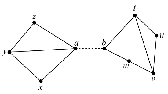
Constructor case (add a bridge): Suppose \(G\) and \(H\) are connected graphs with planar embeddings and disjoint sets of vertices. Let \(\gamma\) be a discrete face of the embedding of \(G\) and suppose that \(\gamma\) begins and ends at vertex \(a\).

Similarly, let \(\delta\) be a discrete face of the embedding of \(H\) that begins and ends at vertex \(b\).

Then the graph obtained by connecting \(G\) and \(H\) with a new edge, \(\langle a - b \rangle\), has a planar embedding whose discrete faces are the union of the discrete faces of \(G\) and \(H\), except that faces \(\gamma\) and \(\delta\) are replaced by one new face

\[\nonumber \gamma \hat{} \langle a - b \rangle \hat{} \delta \hat{} \langle b-a \rangle.\]

This is illustrated in Figure 12.10, where the vertex sequences of the faces of \(G\) and \(H\) are:

\[\nonumber G : \{axyza, axya, ayza\} \quad H : \{btuvwb, btvwb, tuvt\},\]

and after adding the bridge \(\langle a - b \rangle\), there is a single connected graph whose faces have the vertex sequences

\[\nonumber axyz\color{blue}ab\color{black}tuvw\color{blue}ba\color{black}, axya, ayza, btvwb, tuvt.\]

A bridge is simply a cut edge, but in the context of planar embeddings, the bridges are precisely the edges that occur twice on the same discrete face —as opposed to once on each of two faces. Dongles are trees made of bridges; we only use dongles in illustrations, so there’s no need to define them more precisely.

Figure 12.9 The “split a face” case: \(awxbyza\) splits into \(awxba\) and \(abyza\).

Figure 12.10 The “add a bridge” case.

Does It Work?

Yes! In general, a graph is planar because it has a planar drawing according to Definition 12.2.1 if and only if each of its connected components has a planar embedding as specified in Definition 12.2.2. Of course we can’t prove this without an excursion into exactly the kind of continuous math that we’re trying to avoid. But now that the recursive definition of planar graphs is in place, we won’t ever need to fall back on the continuous stuff. That’s the good news.

The bad news is that Definition 12.2.2 is a lot more technical than the intuitively simple notion of a drawing whose edges don’t cross. In many cases it’s easier to stick to the idea of planar drawings and give proofs in those terms. For example, erasing edges from a planar drawing will surely leave a planar drawing. On the other hand, it’s not so obvious, though of course it is true, that you can delete an edge from a planar embedding and still get a planar embedding (see Problem 12.9).

In the hands of experts, and perhaps in your hands too with a little more experience, proofs about planar graphs by appeal to drawings can be convincing and reliable. But given the long history of mistakes in such proofs, it’s safer to work from the precise definition of planar embedding. More generally, it’s also important to see how the abstract properties of curved drawings in the plane can be modelled successfully using a discrete data type.

Where Did the Outer Face Go?

Every planar drawing has an immediately-recognizable outer face —it’s the one that goes to infinity in all directions. But where is the outer face in a planar embedding?

There isn’t one! That’s because there really isn’t any need to distinguish one face from another. In fact, a planar embedding could be drawn with any given face on the outside. An intuitive explanation of this is to think of drawing the embedding on a sphere instead of the plane. Then any face can be made the outside face by “puncturing” that face of the sphere, stretching the puncture hole to a circle around the rest of the faces, and flattening the circular drawing onto the plane.

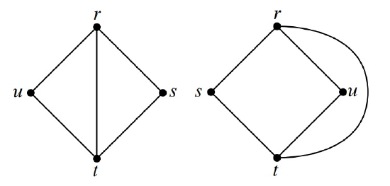
So pictures that show different “outside” boundaries may actually be illustrations of the same planar embedding. For example, the two embeddings shown in Figure 12.11 are really the same —check it: they have the same boundary cycles.

This is what justifies the “add bridge” case in Definition 12.2.2: whatever face is chosen in the embeddings of each of the disjoint planar graphs, we can draw a bridge between them without needing to cross any other edges in the drawing, because we can assume the bridge connects two “outer” faces.

Figure 12.11 Two illustrations of the same embedding.

¹Most texts drop the adjective continuous from the definition of a face as a connected region. We need the adjective to distinguish continuous faces from the discrete faces we’re about to define.

²There is a minor exception to this definition of embedding in the special case when \(G\) is a line graph beginning with \(a\) and ending with \(b\). In this case the cycles into which \(\gamma\) splits are actually the same. That’s because adding edge \(\langle a - b \rangle\) creates a cycle that divides the plane into “inner” and “outer” continuous faces that are both bordered by this cycle. In order to maintain the correspondence between continuous faces and discrete faces in this case, we define the two discrete faces of the embedding to be two “copies” of this same cycle.

³Formally, merge is an operation on walks, not a walk and an edge, so in (\(\ref{12.2.2.}\)), we should have used a walk \(\langle a \langle a - b \rangle b \rangle\) instead of an edge \(\langle a - b \rangle\) and written

\[\nonumber \alpha \hat{} (b \langle b - a \rangle a) \text{ and } (a \langle a - b \rangle b) \hat{} \beta\]