16.3: Strange Dice

The four-step method is surprisingly powerful. Let’s get some more practice with it. Imagine, if you will, the following scenario.

It’s a typical Saturday night. You’re at your favorite pub, contemplating the true meaning of infinite cardinalities, when a burly-looking biker plops down on the stool next to you. Just as you are about to get your mind around \(\text{pow(pow(}\mathbb{R}))\), biker dude slaps three strange-looking dice on the bar and challenges you to a $100 wager. His rules are simple. Each player selects one die and rolls it once. The player with the lower value pays the other player $100.

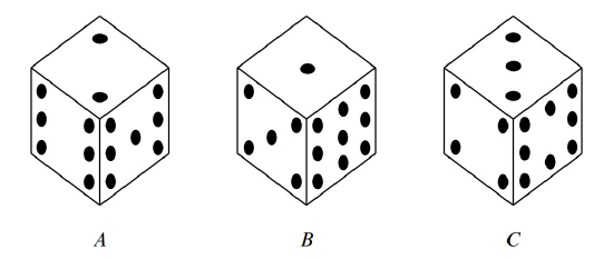
Naturally, you are skeptical, especially after you see that these are not ordinary dice. Each die has the usual six sides, but opposite sides have the same number on them, and the numbers on the dice are different, as shown in Figure 16.6.

Figure 16.6 The strange dice. The number of pips on each concealed face is the same as the number on the opposite face. For example, when you roll die \(A\), the probabilities of getting a 2, 6, or 7 are each \(1/3\).

Biker dude notices your hesitation, so he sweetens his offer: he will pay you $105 if you roll the higher number, but you only need pay him $100 if he rolls higher, and he will let you pick a die first, after which he will pick one of the other two. The sweetened deal sounds persuasive since it gives you a chance to pick what you think is the best die, so you decide you will play. But which of the dice should you choose? Die \(B\) is appealing because it has a 9, which is a sure winner if it comes up. Then again, die \(A\) has two fairly large numbers, and die \(C\) has an 8 and no really small values.

In the end, you choose die \(B\) because it has a 9, and then biker dude selects die \(A\). Let’s see what the probability is that you will win. (Of course, you probably should have done this before picking die \(B\) in the first place.) Not surprisingly, we will use the four-step method to compute this probability.

Die A versus Die B

Step 1: Find the sample space.

The tree diagram for this scenario is shown in Figure 16.7. In particular, the sample space for this experiment are the nine pairs of values that might be rolled with Die \(A\) and Die \(B\):

Figure 16.7 The tree diagram for one roll of die \(A\) versus die \(B\). Die \(A\) wins with probability \(5/9\).

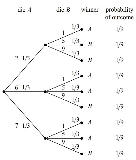
For this experiment, the sample space is a set of nine outcomes:

\[\nonumber S = \{ (2,1), (2,5), (2,9), (6,1), (6,5), (6,9), (7,1), (7,5), (7,9)\}.\]

Step 2: Define events of interest.

We are interested in the event that the number on die \(A\) is greater than the number on die \(B\). This event is a set of five outcomes:

\[\nonumber \{ (2,1), (6,1), (6,5), (7,1), (7,5)\}.\]

These outcomes are marked \(A\) in the tree diagram in Figure 16.7.

Step 3: Determine outcome probabilities.

To find outcome probabilities, we first assign probabilities to edges in the tree diagram. Each number on each die comes up with probability \(1/3\), regardless of the value of the other die. Therefore, we assign all edges probability \(1/3\). The probability of an outcome is the product of the probabilities on the corresponding root-to-leaf path, which means that every outcome has probability \(1/9\). These probabilities are recorded on the right side of the tree diagram in Figure 16.7.

Step 4: Compute event probabilities.

The probability of an event is the sum of the probabilities of the outcomes in that event. In this case, all the outcome probabilities are the same, so we say that the sample space is uniform. Computing event probabilities for uniform sample spaces is particularly easy since you just have to compute the number of outcomes in the event. In particular, for any event \(E\) in a uniform sample space \(S\),

\[\label{16.3.1} \text{Pr}[E] = \dfrac{|E|}{|S|}.\]

In this case, \(E\) is the event that die \(A\) beats die \(B\), so \(|E| = 5\), \(|S| = 9\), and

\[\nonumber \text{Pr}[E] = 5/9.\]

This is bad news for you. Die \(A\) beats die \(B\) more than half the time and, not surprisingly, you just lost $100.

Biker dude consoles you on your “bad luck” and, given that he’s a sensitive guy beneath all that leather, he offers to go double or nothing.¹ Given that your wallet only has $25 in it, this sounds like a good plan. Plus, you figure that choosing die \(A\) will give you the advantage.

So you choose \(A\), and then biker dude chooses \(C\). Can you guess who is more likely to win? (Hint: it is generally not a good idea to gamble with someone you don’t know in a bar, especially when you are gambling with strange dice.)

Die \(A\) versus Die \(C\)

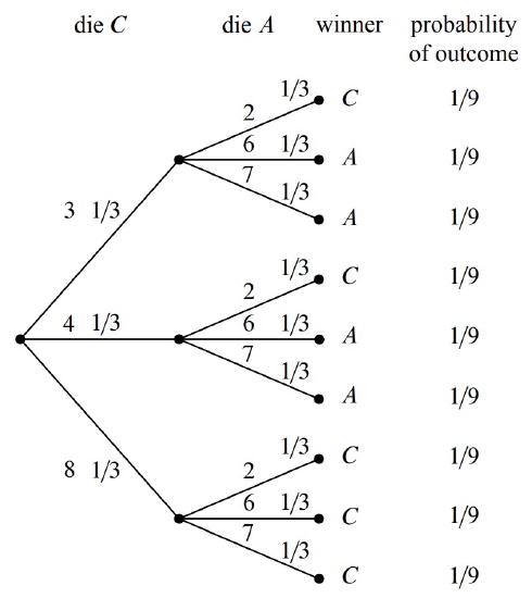
We can construct the tree diagram and outcome probabilities as before. The result is shown in Figure 16.8, and there is bad news again. Die C will beat die A with probability \(5/9\), and you lose once again.

Figure 16.8 The tree diagram for one roll of die \(C\) versus die \(A\). Die \(C\) wins with probability \(5/9\).

You now owe the biker dude $200 and he asks for his money. You reply that you need to go to the bathroom.

Die \(B\) versus Die \(C\)

Being a sensitive guy, biker dude nods understandingly and offers yet another wager. This time, he’ll let you have die \(C\). He’ll even let you raise the wager to $200 so you can win your money back.

This is too good a deal to pass up. You know that die \(C\) is likely to beat die \(A\) and that die \(A\) is likely to beat die \(B\), and so die \(C\) is surely the best. Whether biker dude picks \(A\) or \(B\), the odds would be in your favor this time. Biker dude must really be a nice guy.

So you pick \(C\), and then biker dude picks \(B\). Wait—how come you haven’t caught on yet and worked out the tree diagram before you took this bet? If you do it now, you’ll see by the same reasoning as before that \(B\) beats \(C\) with probability \(5/9\). But surely there is a mistake! How is it possible that

\[\begin{aligned} &C \text{ beats } A \text{ with probability } 5/9, \\ &A \text{ beats } B \text{ with probability } 5/9, \\ &B \text{ beats } C \text{ with probability } 5/9? \end{aligned}\]

The problem is not with the math, but with your intuition. Since \(A\) will beat \(B\) more often than not, and \(B\) will beat \(C\) more often than not, it seems like \(A\) ought to beat \(C\) more often than not, that is, the “beats more often” relation ought to be transitive. But this intuitive idea is simply false: whatever die you pick, biker dude can pick one of the others and be likely to win. So picking first is actually a disadvantage, and as a result, you now owe biker dude $400.

Just when you think matters can’t get worse, biker dude offers you one final wager for $1,000. This time, instead of rolling each die once, you will each roll your die twice, and your score is the sum of your rolls, and he will even let you pick your die second, that is, after he picks his. Biker dude chooses die \(B\). Now you know that die \(A\) will beat die \(B\) with probability \(5/9\) on one roll, so, jumping at this chance to get ahead, you agree to play, and you pick die \(A\). After all, you figure that since a roll of die \(A\) beats a roll of die \(B\) more often that not, two rolls of die \(A\) are even more likely to beat two rolls of die \(B\), right?

Wrong! (Did we mention that playing strange gambling games with strangers in a bar is a bad idea?)

Rolling Twice

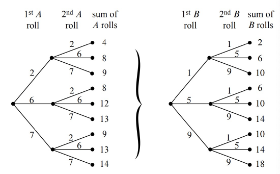
If each player rolls twice, the tree diagram will have four levels and \(3^4 = 81\) outcomes. This means that it will take a while to write down the entire tree diagram. But it’s easy to write down the first two levels as in Figure 16.9(a) and then notice that the remaining two levels consist of nine identical copies of the tree in Figure 16.9(b).

Figure 16.9 Parts of the tree diagram for die \(B\) versus die \(A\) where each die is rolled twice. The first two levels are shown in (a). The last two levels consist of nine copies of the tree in (b).

The probability of each outcome is \((1/3)^4 = 1/81\) and so, once again, we have a uniform probability space. By equation (\ref{16.3.1}), this means that the probability that \(A\) wins is the number of outcomes where \(A\) beats \(B\) divided by 81.

To compute the number of outcomes where \(A\) beats \(B\), we observe that the two rolls of die \(A\) result in nine equally likely outcomes in a sample space \(S_A\) in which the two-roll sums take the values

\[\nonumber (4,8,8,9,9,12,13,13,14).\]

Likewise, two rolls of die \(B\) result in nine equally likely outcomes in a sample space \(S_B\) in which the two-roll sums take the values

\[\nonumber (2,6,6,10,10,10,14,14,18).\]

We can treat the outcome of rolling both dice twice as a pair\((x, y) \in S_A \times S_B\), where \(A\) wins iff the sum of the two \(A\)-rolls of outcome \(x\) is larger the sum of the two \(B\)-rolls of outcome \(y\). If the \(A\)-sum is 4, there is only one \(y\) with a smaller \(B\)-sum, namely, when the \(B\)-sum is 2. If the \(A\)-sum is 8, there are three \(y\)’s with a smaller \(B\)-sum, namely, when the \(B\)-sum is 2 or 6. Continuing the count in this way, the number of pairs\((x, y)\) for which the \(A\)-sum is larger than the \(B\)-sum is

\[\nonumber 1 + 3 + 3 + 3 + 3 + 6 + 6 + 6 + 6 = 37.\]

A similar count shows that there are 42 pairs for which \(B\)-sum is larger than the \(A\)-sum, and there are two pairs where the sums are equal, namely, when they both equal 14. This means that \(A\) loses to \(B\) with probability \(42/81 > 1/2\) and ties with probability \(2/81\). Die \(A\) wins with probability only \(37/81\).

How can it be that \(A\) is more likely than \(B\) to win with one roll, but \(B\) is more likely to win with two rolls? Well, why not? The only reason we’d think otherwise is our unreliable, untrained intuition. (Even the authors were surprised when they first learned about this, but at least they didn’t lose $1400 to biker dude.) In fact, the die strength reverses no matter which two die we picked. So for one roll,

\[A \succ B \succ C \succ A,\]

but for two rolls,

\[A \prec B \prec C \prec A,\]

where we have used the symbols \(\succ\) and \(\prec\) to denote which die is more likely to result in the larger value.

The weird behavior of the three strange dice above generalizes in a remarkable way: there are arbitrarily large sets of dice which will beat each other in any desired pattern according to how many times the dice are rolled.²

² TBA - Reference Ron Graham paper.