15.4: Plotting Univariate Data

There are basically two useful ways of plotting a Series with univariate data. In one, you care about the specific labels (i.e. keys, or “index”) of the values in the Series, and you want them to be prominent in the plot. In the other, you don’t; you just want to show the values themselves, so you can visualize how they are distributed irrespective of what label they might have.

Let’s do the first one first.

Bar Charts of Labeled Data

Let’s read a data set on the world countries with the highest GDP (Gross Domestic Product). Here’s a CSV file called gdp.csv¹ :

Code \(\PageIndex{1}\) (Python):

Nation,Trillions

Italy,2.26

Germany,4.42

Brazil,2.26

United States,21.41

France,3.06

Canada,1.91

Japan,5.36

China,15.54

India,3.16

United Kingdom,3.02

We’ll read that into a Series using our technique:

Code \(\PageIndex{2}\) (Python):

gdp = pd.read_csv('gdp.csv', squeeze=True, index_col=0, header=None)

print(gdp)

| 0

| Nation Trillions

| Italy 2.26

| Germany 4.42

| Brazil 2.26

| United States 21.41

| France 3.06

| Canada 1.91

| Japan 5.36

| China 15.54

| India 3.16

| United Kingdom 3.02

| Name: 1, dtype: object

and now, we can visualize the relative sizes of these economies with the .plot() method. The .plot() method takes, among other things, a “kind” argument which specifies what kind of plot you want. In this case, a bar chart is the correct thing:

Code \(\PageIndex{3}\) (Python):

gdp.plot(kind='bar')

There are a zillion ways to customize these plots, and I’ll only mention a very, very few. A more complete list of options is available by Googling, or going to https://matplotlib.org/3.1.1/api/_as_ gen/matplotlib.pyplot.plot.html

For instance, to make all the bars the same color, we can pass “color="blue"”. Sorting the values is something we already know how to do, with .sort_values():

Code \(\PageIndex{4}\) (Python):

gdp.sort_values(ascending=False).plot(kind='bar')

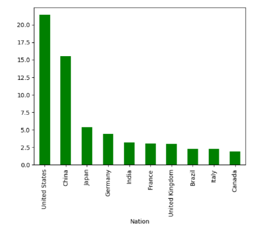
You see what I mean about “caring about the labels/keys/index” for this sort of plot: if we hadn’t labeled the bars, the plot would tell us nothing useful.

I’m sure you’ve seen lots of bar charts in your life, so this is nothing new. But consider how much information is embedded in this infographic. Not only can we tell that the U.S. and China are the two biggest economies, we can tell that they are far and away the two biggest, with Japan and Germany (the next two highest) only a fraction.

Bar Charts of Occurrence Counts

A very common special case of a bar chart is one where we combine it with the .value_counts() method. Let’s go back to Taylor vs. Katy:

Code \(\PageIndex{5}\) (Python):

print(faves)

| 0 Katy Perry

| 1 Rihanna

| 2 Justin Bieber

| 3 Drake

| 4 Rihanna

| 5 Taylor Swift

| 6 Adele

| 7 Adele

| 8 Taylor Swift

| 9 Justin Bieber

| ...

| 1395 Katy Perry

| dtype: object

It would be useful to see an infographic on how popular each celebrity is, and combining .value_counts() and .plot() makes it a snap:

Code \(\PageIndex{6}\) (Python):

faves.value_counts().plot(kind='bar',color="orange")

The .sort_values() method wasn’t needed here, because our friend .value_counts() already returns its answer in decreasing numerical order. If we wanted the bars in alphabetical order instead, we’d just sort the Series by index before plotting:

Code \(\PageIndex{7}\) (Python):

faves.value_counts().sort_index().plot(kind='bar', color="purple")

These long lines with lots of strung-together methods are concise, but can also be confusing. It’s always an option to use temporary variables to store the intermediate results instead:

Code \(\PageIndex{8}\) (Python):

counts = faves.value_counts()

alphbetical_counts = counts.sort_index()

alphbetical_counts.plot(kind='bar',color="purple")

Just a matter of preference.