28.1: Decision Trees in Python

Last updated
Save as PDF

Page ID: 88805

\( \newcommand{\vecs}[1]{\overset { \scriptstyle \rightharpoonup} {\mathbf{#1}} } \) \( \newcommand{\vecd}[1]{\overset{-\!-\!\rightharpoonup}{\vphantom{a}\smash {#1}}} \)\(\newcommand{\id}{\mathrm{id}}\) \( \newcommand{\Span}{\mathrm{span}}\) \( \newcommand{\kernel}{\mathrm{null}\,}\) \( \newcommand{\range}{\mathrm{range}\,}\) \( \newcommand{\RealPart}{\mathrm{Re}}\) \( \newcommand{\ImaginaryPart}{\mathrm{Im}}\) \( \newcommand{\Argument}{\mathrm{Arg}}\) \( \newcommand{\norm}[1]{\| #1 \|}\) \( \newcommand{\inner}[2]{\langle #1, #2 \rangle}\) \( \newcommand{\Span}{\mathrm{span}}\) \(\newcommand{\id}{\mathrm{id}}\) \( \newcommand{\Span}{\mathrm{span}}\) \( \newcommand{\kernel}{\mathrm{null}\,}\) \( \newcommand{\range}{\mathrm{range}\,}\) \( \newcommand{\RealPart}{\mathrm{Re}}\) \( \newcommand{\ImaginaryPart}{\mathrm{Im}}\) \( \newcommand{\Argument}{\mathrm{Arg}}\) \( \newcommand{\norm}[1]{\| #1 \|}\) \( \newcommand{\inner}[2]{\langle #1, #2 \rangle}\) \( \newcommand{\Span}{\mathrm{span}}\)\(\newcommand{\AA}{\unicode[.8,0]{x212B}}\)

Our decision tree pictures from chapter 27 were quite illustrative, but of course to actually automate something, we have to write code rather than draw pictures. What would Figure 27.1 (p. 273) look like in Python code? It’s actually pretty simple, although there’s a lot of nested indentation. See if you can follow the flow in Figure 28.1.1.

Here we’re defining a function called predict() that takes three arguments, one for each feature value. The eye-popping set of if/elif/else statements looks daunting at first, but when you scrutinize it you’ll realize it perfectly reflects the structure of the purple diagram. Each time we go down one level of the tree, we indent one tab to the right. The body of the “if major == 'PSYC':” statement is very short because the left-most branch of the tree (for Psychology) is very simple. The “elif major == 'CPSC':” body, by contrast, has lots of nested internal structure precisely because the right-most branch of the tree (for Computer Science) is complex. Etc.

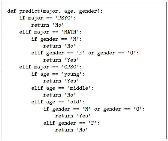
Figure \(\PageIndex(1)\): A Python implementation of the decision tree in Figure 27.2.1

If we call this function, it will give us exactly the same predictions we calculated by hand on p. 273:

Code \(\PageIndex{1}\) (Python):

print(predict('PSYC','M','old'))

print(predict('MATH','O','young'))

print(predict('CPSC','F','old'))

Output:

| No

| Yes

| No