3.13: Standing Waves
- Page ID
- 6279

\( \newcommand{\vecs}[1]{\overset { \scriptstyle \rightharpoonup} {\mathbf{#1}} } \)
\( \newcommand{\vecd}[1]{\overset{-\!-\!\rightharpoonup}{\vphantom{a}\smash {#1}}} \)
\( \newcommand{\dsum}{\displaystyle\sum\limits} \)
\( \newcommand{\dint}{\displaystyle\int\limits} \)
\( \newcommand{\dlim}{\displaystyle\lim\limits} \)
\( \newcommand{\id}{\mathrm{id}}\) \( \newcommand{\Span}{\mathrm{span}}\)
( \newcommand{\kernel}{\mathrm{null}\,}\) \( \newcommand{\range}{\mathrm{range}\,}\)
\( \newcommand{\RealPart}{\mathrm{Re}}\) \( \newcommand{\ImaginaryPart}{\mathrm{Im}}\)
\( \newcommand{\Argument}{\mathrm{Arg}}\) \( \newcommand{\norm}[1]{\| #1 \|}\)
\( \newcommand{\inner}[2]{\langle #1, #2 \rangle}\)
\( \newcommand{\Span}{\mathrm{span}}\)
\( \newcommand{\id}{\mathrm{id}}\)
\( \newcommand{\Span}{\mathrm{span}}\)
\( \newcommand{\kernel}{\mathrm{null}\,}\)
\( \newcommand{\range}{\mathrm{range}\,}\)
\( \newcommand{\RealPart}{\mathrm{Re}}\)
\( \newcommand{\ImaginaryPart}{\mathrm{Im}}\)
\( \newcommand{\Argument}{\mathrm{Arg}}\)
\( \newcommand{\norm}[1]{\| #1 \|}\)
\( \newcommand{\inner}[2]{\langle #1, #2 \rangle}\)
\( \newcommand{\Span}{\mathrm{span}}\) \( \newcommand{\AA}{\unicode[.8,0]{x212B}}\)
\( \newcommand{\vectorA}[1]{\vec{#1}} % arrow\)
\( \newcommand{\vectorAt}[1]{\vec{\text{#1}}} % arrow\)
\( \newcommand{\vectorB}[1]{\overset { \scriptstyle \rightharpoonup} {\mathbf{#1}} } \)
\( \newcommand{\vectorC}[1]{\textbf{#1}} \)
\( \newcommand{\vectorD}[1]{\overrightarrow{#1}} \)
\( \newcommand{\vectorDt}[1]{\overrightarrow{\text{#1}}} \)
\( \newcommand{\vectE}[1]{\overset{-\!-\!\rightharpoonup}{\vphantom{a}\smash{\mathbf {#1}}}} \)
\( \newcommand{\vecs}[1]{\overset { \scriptstyle \rightharpoonup} {\mathbf{#1}} } \)
\(\newcommand{\longvect}{\overrightarrow}\)
\( \newcommand{\vecd}[1]{\overset{-\!-\!\rightharpoonup}{\vphantom{a}\smash {#1}}} \)
\(\newcommand{\avec}{\mathbf a}\) \(\newcommand{\bvec}{\mathbf b}\) \(\newcommand{\cvec}{\mathbf c}\) \(\newcommand{\dvec}{\mathbf d}\) \(\newcommand{\dtil}{\widetilde{\mathbf d}}\) \(\newcommand{\evec}{\mathbf e}\) \(\newcommand{\fvec}{\mathbf f}\) \(\newcommand{\nvec}{\mathbf n}\) \(\newcommand{\pvec}{\mathbf p}\) \(\newcommand{\qvec}{\mathbf q}\) \(\newcommand{\svec}{\mathbf s}\) \(\newcommand{\tvec}{\mathbf t}\) \(\newcommand{\uvec}{\mathbf u}\) \(\newcommand{\vvec}{\mathbf v}\) \(\newcommand{\wvec}{\mathbf w}\) \(\newcommand{\xvec}{\mathbf x}\) \(\newcommand{\yvec}{\mathbf y}\) \(\newcommand{\zvec}{\mathbf z}\) \(\newcommand{\rvec}{\mathbf r}\) \(\newcommand{\mvec}{\mathbf m}\) \(\newcommand{\zerovec}{\mathbf 0}\) \(\newcommand{\onevec}{\mathbf 1}\) \(\newcommand{\real}{\mathbb R}\) \(\newcommand{\twovec}[2]{\left[\begin{array}{r}#1 \\ #2 \end{array}\right]}\) \(\newcommand{\ctwovec}[2]{\left[\begin{array}{c}#1 \\ #2 \end{array}\right]}\) \(\newcommand{\threevec}[3]{\left[\begin{array}{r}#1 \\ #2 \\ #3 \end{array}\right]}\) \(\newcommand{\cthreevec}[3]{\left[\begin{array}{c}#1 \\ #2 \\ #3 \end{array}\right]}\) \(\newcommand{\fourvec}[4]{\left[\begin{array}{r}#1 \\ #2 \\ #3 \\ #4 \end{array}\right]}\) \(\newcommand{\cfourvec}[4]{\left[\begin{array}{c}#1 \\ #2 \\ #3 \\ #4 \end{array}\right]}\) \(\newcommand{\fivevec}[5]{\left[\begin{array}{r}#1 \\ #2 \\ #3 \\ #4 \\ #5 \\ \end{array}\right]}\) \(\newcommand{\cfivevec}[5]{\left[\begin{array}{c}#1 \\ #2 \\ #3 \\ #4 \\ #5 \\ \end{array}\right]}\) \(\newcommand{\mattwo}[4]{\left[\begin{array}{rr}#1 \amp #2 \\ #3 \amp #4 \\ \end{array}\right]}\) \(\newcommand{\laspan}[1]{\text{Span}\{#1\}}\) \(\newcommand{\bcal}{\cal B}\) \(\newcommand{\ccal}{\cal C}\) \(\newcommand{\scal}{\cal S}\) \(\newcommand{\wcal}{\cal W}\) \(\newcommand{\ecal}{\cal E}\) \(\newcommand{\coords}[2]{\left\{#1\right\}_{#2}}\) \(\newcommand{\gray}[1]{\color{gray}{#1}}\) \(\newcommand{\lgray}[1]{\color{lightgray}{#1}}\) \(\newcommand{\rank}{\operatorname{rank}}\) \(\newcommand{\row}{\text{Row}}\) \(\newcommand{\col}{\text{Col}}\) \(\renewcommand{\row}{\text{Row}}\) \(\newcommand{\nul}{\text{Nul}}\) \(\newcommand{\var}{\text{Var}}\) \(\newcommand{\corr}{\text{corr}}\) \(\newcommand{\len}[1]{\left|#1\right|}\) \(\newcommand{\bbar}{\overline{\bvec}}\) \(\newcommand{\bhat}{\widehat{\bvec}}\) \(\newcommand{\bperp}{\bvec^\perp}\) \(\newcommand{\xhat}{\widehat{\xvec}}\) \(\newcommand{\vhat}{\widehat{\vvec}}\) \(\newcommand{\uhat}{\widehat{\uvec}}\) \(\newcommand{\what}{\widehat{\wvec}}\) \(\newcommand{\Sighat}{\widehat{\Sigma}}\) \(\newcommand{\lt}{<}\) \(\newcommand{\gt}{>}\) \(\newcommand{\amp}{&}\) \(\definecolor{fillinmathshade}{gray}{0.9}\)A standing wave consists of waves moving in opposite directions. These waves add to make a distinct magnitude variation as a function of distance that does not vary in time.
To see how this can happen, first consider that an incident wave \(V_0^+ e^{-j\beta z}\), which is traveling in the \(+z\) axis along a lossless transmission line. Associated with this wave is a reflected wave \(V_0^- e^{+j\beta z}=\Gamma V_0^+ e^{+j\beta z}\), where \(\Gamma\) is the voltage reflection coefficient. These waves add to make the total potential
\[\begin{split} \widetilde{V}(z) & = V_0^+ e^{-j\beta z} + \Gamma V_0^+ e^{+j\beta z} \\ & = V_0^+ \left( e^{-j\beta z} + \Gamma e^{+j\beta z} \right) \end{split} \nonumber \]
The magnitude of \(\widetilde{V}(z)\) is most easily found by first finding \(|\widetilde{V}(z)|^2\), which is:
\begin{aligned}
& \tilde{V}(z) \tilde{V}^{*}(z) \\
=&\left|V_{0}^{+}\right|^{2}\left(e^{-j \beta z}+\Gamma e^{+j \beta z}\right)\left(e^{-j \beta z}+\Gamma e^{+j \beta z}\right)^{*} \\
=&\left|V_{0}^{+}\right|^{2}\left(e^{-j \beta z}+\Gamma e^{+j \beta z}\right)\left(e^{+j \beta z}+\Gamma^{*} e^{-j \beta z}\right) \\
=&\left|V_{0}^{+}\right|^{2}\left(1+|\Gamma|^{2}+\Gamma e^{+j 2 \beta z}+\Gamma^{*} e^{-j 2 \beta z}\right)
\end{aligned}
Let \(\phi\) be the phase of \(\Gamma\); i.e.,
\[\Gamma = \left|\Gamma\right|e^{j\phi} \nonumber \]
Then, continuing from the previous expression:
\begin{aligned}
&\left|V_{0}^{+}\right|^{2}\left(1+|\Gamma|^{2}+|\Gamma| e^{+j(2 \beta z+\phi)}+|\Gamma| e^{-j(2 \beta z+\phi)}\right) \\
=&\left|V_{0}^{+}\right|^{2}\left(1+|\Gamma|^{2}+|\Gamma|\left[e^{+j(2 \beta z+\phi)}+e^{-j(2 \beta z+\phi)}\right]\right)
\end{aligned}
The quantity in square brackets can be reduced to a cosine function using the identity
\[\cos\theta = \frac{1}{2}\left[e^{j\theta}+e^{-j\theta}\right] \nonumber \]
yielding: \[|V_0^+|^2 \left[ 1 + \left|\Gamma\right|^2 + 2\left|\Gamma\right| \cos\left( 2\beta z + \phi \right) \right] \nonumber \]
Recall that this is \(|\widetilde{V}(z)|^2\). \(|\widetilde{V}(z)|\) is therefore the square root of the above expression:
\[\left|\widetilde{V}(z)\right| = |V_0^+| \sqrt{ 1 + \left|\Gamma\right|^2 + 2\left|\Gamma\right| \cos\left( 2\beta z + \phi \right) } \nonumber \]
Thus, we have found that the magnitude of the resulting total potential varies sinusoidally along the line. This is referred to as a standing wave because the variation of the magnitude of the phasor resulting from the interference between the incident and reflected waves does not vary with time.
We may perform a similar analysis of the current, leading to: \[\left|\widetilde{I}(z)\right| = \frac{|V_0^+|}{Z_0} \sqrt{ 1 + \left|\Gamma\right|^2 - 2\left|\Gamma\right| \cos\left( 2\beta z + \phi \right) } \nonumber \]
Again we find the result is a standing wave.
Now let us consider the outcome for a few special cases.
Matched load. When the impedance of the termination of the transmission line, \(Z_L\), is equal to the characteristic impedance of the transmission line, \(Z_0\), \(\Gamma=0\) and there is no reflection. In this case, the above expressions reduce to \(|\widetilde{V}(z)| = |V_0^+|\) and \(|\widetilde{I}(z)| = |V_0^+|/Z_0\), as expected.
Open or Short-Circuit. In this case, \(\Gamma=\pm1\) and we find:
\[\left|\widetilde{V}(z)\right| = |V_0^+| \sqrt{ 2 + 2\cos\left( 2\beta z + \phi \right) } \nonumber \]
\[\left|\widetilde{I}(z)\right| = \frac{|V_0^+|}{Z_0} \sqrt{ 2 - 2\cos\left( 2\beta z + \phi \right) } \nonumber \]
where \(\phi=0\) for an open circuit and \(\phi=\pi\) for a short circuit. The result for an open circuit termination is shown in Figure \(\PageIndex{1}\)(a) (potential) and \(\PageIndex{1}\)(b) (current). The result for a short circuit termination is identical except the roles of potential and current are reversed. In either case, note that voltage maxima correspond to current minima, and vice versa.
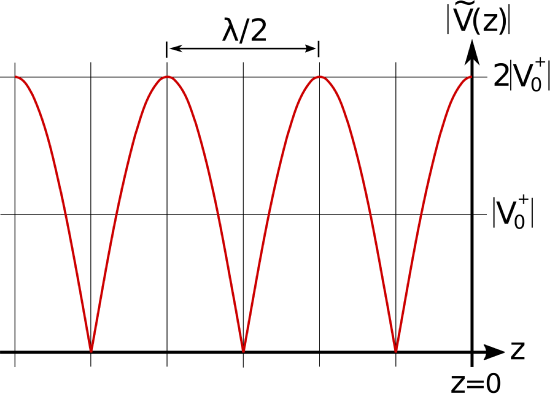
(a) Potential.
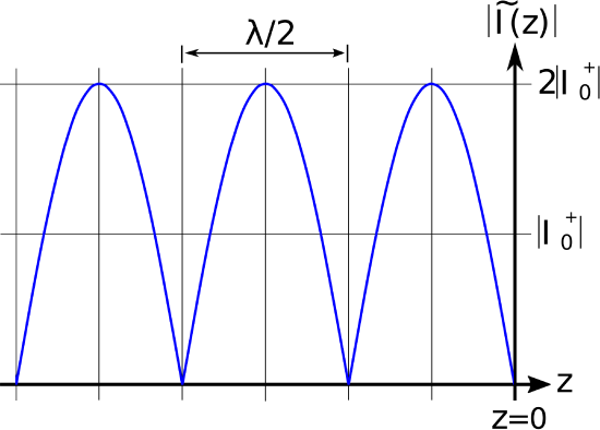
(b) Current.
Figure \(\PageIndex{1}\): Standing wave associated with an opencircuit termination at \(z = 0\) (incident wave arrives from left).
Also note:
The period of the standing wave is \(\lambda/2\); i.e., one-half of a wavelength.
This can be confirmed as follows. First, note that the frequency argument of the cosine function of the standing wave is \(2\beta z\). This can be rewritten as \(2\pi\left(\beta/\pi\right)z\), so the frequency of variation is \(\beta/\pi\) and the period of the variation is \(\pi/\beta\). Since \(\beta=2\pi/\lambda\), we see that the period of the variation is \(\lambda/2\). Furthermore, this is true regardless of the value of \(\Gamma\).
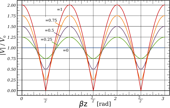
Mismatched loads. A common situation is that the termination is neither perfectly-matched (\(\Gamma=0\)) nor an open/short circuit (\(\left|\Gamma\right|=1\)). Examples of the resulting standing waves are shown in Figure \(\PageIndex{2}\).