2.8: Lumped Parameter Electroquasistatic Elements

Lumped parameter electromechanical models are sufficiently practical that they warrant detailed examination.\(^1\) Even though the electromechanical coupling may be of a definitely continuum and distributed nature, it is most often the case that interest is in inputs and outputs at discrete terminal pairs. This section reviews the definition of energy storage elements in EQS systems.

An abstract representation of a system of perfectly conducting electrodes, each having a potential \(v_i\) relative to a reference electrode, is shown in Figure 2.11.1. Not only are the electrodes and their connecting leads perfectly conducting, but the environment surrounding them is perfectly insulating.

Figure 2.11.1 Schematic view of an electrode system consisting of n electrodes composed of perfect conductors and immersed in a perfectly insulating medium.

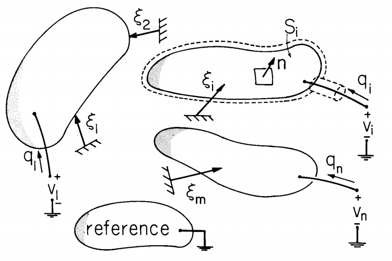
The charge on each of the n electrodes is the free charge density integrated over a volume the electrode:

\[ q_i \equiv \int_{V_i} \rho_f dV = \oint_{S_i} \overrightarrow{D} \cdot \overrightarrow{n} da \label{1} \]

The total charge on an electrode is indicated by an arrow pointing toward the electrode from the terminal pair attached to that electrode. The associated voltage is defined in terms of the electric field and the potential by

\[ v_i = - \int_{ref}^{(i)} \overrightarrow{E} \cdot \overrightarrow{d}l = \phi_i - \phi_{ref} = \phi_i \label{2} \]

This relation is justified because the electric field is irrotational and hence the negative gradient of \(\phi\)

Given the geometry of the electrodes at a certain instant in time, displacements \(\xi_1 ... \xi_j ...\xi_m\) are known, and the condition that the field be irrotational and satisfy Gauss' law leads to equations that can in principle be used to determine the charges on the individual electrodes at a given instant:

\[ q_i = q_i (v_1...v_n, \quad \xi_1...\xi_m) \label{3} \]

If the dielectrics are electrically linear in the sense that \(\overrightarrow{D} = \varepsilon \overrightarrow{E}\), where \(\varepsilon\) is a function of position but not of time or the field, then it is useful to define a capacitance

\[ C_{ij} = \frac{q_i}{v_j} \Big|_{v_{i \neq j} = 0} = \frac{\oint_{S_i} \varepsilon \overrightarrow{E} \cdot \overrightarrow{n} da}{-\int_{ref}^{j} \overrightarrow{E} \cdot \overrightarrow{d}l} \label{4} \]

The capacitance of the ith electrode relative to the jth electrode is the charge on the ith electrode per unit voltage on the jth electrode, with all other electrodes held at zero voltage. The capacitance is useful as a parameter because the charge on an electrode in a linear dielectric is proportional to the voltage itself; hence, the capacitance is purely a function of the electrical properties of the system and the geometry:

\[ q_i = \sum_{j=1}^{n} C_{ij} v_j, \quad C_{ij} = C_{ij} (\xi_1...\xi_m) \label{5} \]

To define the capacitance as with Eqs. \ref{4} and \ref{5}, no reference is required to the time rate o change. In these relations \(q_i\), \(v_i\), and \(\xi_i\) can all be functions of time. The dynamics enter by virtue of conservation of charge, which can be written for a volume including the ith electrode as (Equation 2.7.3a):

\[ \oint_{S_i} \overrightarrow{J_f^{'}} \cdot \overrightarrow{n} da = - \frac{d}{dt} \int_{V_i} \rho_f dV \label{6} \]

The quantity on the right in this expression is the negative of the time rate of change of the total free charge on the ith electrode. The only free current density normal to a surface enclosing the electrode is that through the wire itself. Note that the normal vector is defined as outward from this surface while a positive current through the wire flows inward. Hence, the left-hand side of Equation \ref{6} becomes the negative of the total current at the ith electrical terminal pair:

\[ i_i = \frac{dq_i}{dt} \label{7} \]

With the charge given as a function of the voltages and the geometry by Equation \ref{3}, or in particular by Equation \ref{5}, Equation \ref{7} can be used to compute the current flowing into a given terminal of the electrode system.

---

1. H. H. Woodson and J. R. Melcher, Electromechanical Dynamics, Vol. I, John Wiley & Sons, New York, 1968.