2.13: Flux-Potential Transfer Relations for Laplacian Fields

It is often convenient in the modeling of a physical system to divide the volume of interest into regions having uniform properties. Surfaces enclosing these regions are often planar, cylindrical or spherical, with the volume then taking the form of a planar layer, a cylindrical annulus or a spherical shell. Such volumes and bounding surfaces are illustrated in Tables 2.16.1-3. The question answered in this section is: given the potential on the bounding surfaces, what are the associated normal flux densities? Of immediate interest is the relation of the electric potentials to the normal displacement vectors. But also treated in this section is the relation of the magnetic potential to the normal magnetic flux densities. First the electroquasistatic fields are considered, and then the magnetoquasistatic relations follow by analogy.

Electric Fields: If any one of the regions shown in Tables 2.16.1-3 is filled with insulating charge-free \((\rho_f = 0)\) material of uniform permittivity \(\varepsilon\),

\[ \overrightarrow{P} = (\varepsilon - \varepsilon_o) \overrightarrow{E}, \quad \overrightarrow{D} = \varepsilon \overrightarrow{E} \label{1} \]

the governing field equations are Gauss' law, Equation 2.3.23a,

\[ \nabla \cdot \overrightarrow{D} = 0 \label{2} \]

and the condition that \(\overrightarrow{E}\) be irrotational, Equation 2.3.24a. The latter is equivalent to

\[ \overrightarrow{E} = -\nabla \phi \label{3} \]

Thus, the potential distribution within a volume is described by Laplace's equation

\[ \nabla^2 \phi = 0 \label{4} \]

In terms of \(\phi\),

\[ \overrightarrow{D} = -\varepsilon \nabla \phi \label{5} \]

Magnetic Fields: For magnetoquasistatic fields in an insulating region \((J_f = 0)\) of uniform permeability

\[ \overrightarrow{M} = (\frac{\mu}{\mu_o} -1) \overrightarrow{H}; \quad \overrightarrow{B} = \mu \overrightarrow{H} \label{6} \]

Thus, from Ampere's law, Equation 2.3.23b, \(\overrightarrow{H}\) is irrotational and it is appropriate to define a magnetic potential \(\psi\):

\[ \overrightarrow{H} = -\nabla \psi \label{7} \]

In addition. there is Equation 2.3.24b:

\[ \nabla \cdot \overrightarrow{B} = 0 \label{8} \]

Thus, the potential again satisfies Laplace's equation

\[ \nabla^2 \psi = 0 \label{9} \]

and in terms of \(\psi\), the magnetic flux density is

\[ \overrightarrow{B} = -\mu \nabla \psi \label{10} \]

Comparison of the last two relations to Eqs. \ref{4} and \ref{5} shows that relations now derived for the electric fields can be carried over to describe the magnetic fields by making the identification \((\phi,\overrightarrow{D},\varepsilon) \rightarrow (\psi,\overrightarrow{B}, \mu)\)

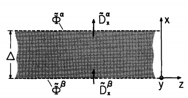
Planar Layer: Bounding surfaces at \(x = \Delta\) and \(x = 0\), respectively denoted by \(\alpha\) and \(\beta\), are shown in Table 2.16.1. So far as developments in this section are concerned, these are not physical boundaries They are simply surfaces at which the potentials are respectively

\[ \phi(\Delta,y,z,t) = RE \tilde{\phi}^{\alpha} (t) exp[-j(k_y y + k_z z)]; \quad \phi(0,y,z,t) = Re \tilde{\phi}^{\beta} (t) exp[-j(k_y y + k_z z)] \label{11} \]

Table 2.16.1. Flux-potential -transfer relations for planar layer in terms of electric potential and normal displacement \((\phi,D_x)\). To obtain magnetic relations, substitute \((\phi,D_x,\varepsilon) \rightarrow (\psi,B_x,\mu)\).

Planar Layer
	\[\begin{bmatrix} \tilde{D}_x^{\alpha}\\ \tilde{D}_x^{\beta} \end{bmatrix} = \varepsilon \gamma \begin{bmatrix} -coth(\gamma \Delta) & \frac{1}{sinh(\gamma \Delta)} \\ \frac{-1}{sinh(\gamma \Delta)} & coth(\gamma \Delta) \end{bmatrix} \begin{bmatrix} \tilde{\phi}^{\alpha}\\ \tilde{\phi}^{\beta} \end{bmatrix} \tag{a} \]
\[ \phi = RE \tilde{\phi}(x,t) e^{-j(k_y y + k_z z)} \nonumber \] \[ \gamma \equiv \sqrt{k_y^2 + k_z^2} \nonumber \]	\[\begin{bmatrix} \tilde{\phi}^{\alpha}\\ \tilde{\phi}^{\beta} \end{bmatrix} = \frac{1}{\varepsilon \gamma} \begin{bmatrix} -coth(\gamma \Delta) & \frac{1}{sinh(\gamma \Delta)} \\ \frac{-1}{sinh(\gamma \Delta)} & coth(\gamma \Delta) \end{bmatrix} \begin{bmatrix} \tilde{D}_x^{\alpha}\\ \tilde{D}_x^{\beta} \end{bmatrix} \tag{b} \]

These will be recognized as generalizations of the complex amplitudes introduced with Equation 2.15.1. That the potentials at the a and $ surfaces can be quite general follows from the discussion of Sec. 2.15, which shows that the following arguments apply when I is a spatial Fourier amplitude or a Fourier transform.

In view of the surface potential distributions, solutions to Equation \ref{4} are assumed to take the form

\[ \phi = RE \tilde{\phi} (x,t) exp[-j(k_y y + k_z z)] \label{12} \]

Substitution shows that

\[ \frac{d^2 \tilde{\phi}}{dx^2} - \gamma^2 \tilde{\phi} = 0; \quad \gamma = \sqrt{k_y^2 + k_z^2} \label{13} \]

Solutions of this equation are linear combinations of \(e^{\pm \gamma x}\) or alternatively of \(sinh\, \gamma x\) and \(cosh\, \gamma x\). With \(\tilde{\phi}_1\) and \(\tilde{\phi}_2\)arbitrary functions of time, the solution takes the form

\[ \tilde{\phi} = \tilde{\phi}_1\, sinh\, \gamma x + \tilde{\phi}_2\, cosh\, \gamma x \label{14} \]

The two coefficients are determined by requiring that the conditions of Equation \ref{11} be satisfied. For the simple situation at hand, an instructive alternative to performing the algebra necessary to evaluate \(\tilde{\phi}_1, \tilde{\phi}_2\) consists in recognizing that a linear combination of the two solutions in Equation \ref{14} is \(sinh\, \gamma(x-\Delta)\). Thus, the solution can be written as the sum of solutions that are individually zero on one or the other of the bounding surfaces. By inspection, it follows that

\[ \tilde{\phi} = \tilde{\phi}^{\alpha} \frac{sinh\, \gamma x}{sinh\, \gamma \Delta} - \tilde{\phi}^{\beta} \frac{sinh\, \gamma (x - \Delta)}{sinh\, \gamma \Delta} \label{15} \]

From Eqs. \ref{5} and \ref{15}, \(\overrightarrow{D}\) can be determined:

\[ \overrightarrow{D}_x = -\varepsilon \frac{\partial{\phi}}{\partial{x}} = -\varepsilon Re \gamma \Bigg[ \tilde{\phi}^{\alpha} \frac{cosh\, \gamma x}{sinh\, \gamma \Delta} - \tilde{\phi}^{\beta} \frac{cosh\, \gamma (x-\Delta)}{sinh\, \gamma \Delta} \Bigg] e^{-j(k_y y + k_z z)} \label{16} \]

Evaluation of this equation at \(x = \Delta\) gives the displacement vector normal to the \(\alpha\) surface, with complex amplitude \(\tilde{D}_x^{\alpha}\). Similarly, evaluated at \(x = 0\), Equation \ref{16} gives \(\tilde{D}_x^{\beta}\). The components of the "flux" \((\tilde{D}_x^{\alpha},\tilde{D}_x^{\beta})\) are now determined, given the respective potentials \((\tilde{\phi}^{\alpha},\tilde{\phi}^{\beta})\). The transfer relations, Equation (a) of Table 2.16.1, summarize what is found. These relations can be solved for any pair of variables as a function of the remaining pair. The inverse transfer relations are also summarized for reference in Table 2.16.1, Equation (b)

Figure 2.16.1. (a) Transfer coefficients as a function of \(\Delta \gamma \equiv \Delta \sqrt{k_y^2 + k_z^2} \) (b) Distribution of \(\phi\) across layer.

That the layer is essentially a distributed capacitance (inductance) is emphasized by drawing attention to the analogy between the transfer relations and constitutive laws for a system of linear capacitors (inductors). For a two-terminal-pair system, Equation 2.11.5 comprises two terminal charges \((q_1,q_2)\) expressed as linear functions of the terminal voltages \((v_1,v_2)\). Analogously, the \((D_x^{\alpha},D_x^{\beta})\) which have units of charge per unit area and an arbitrary time dependence) are given as linear functions of the potentials by Equation (a) of Table 2.16.1. A similar analogy exists between Equation 2.12.5, expressing \((\lambda_1, \lambda_2)\) as functions of \((i_1,i_2)\), and the transfer relations between \((\beta_x^{\alpha}, \beta_x^{\beta})\) (units of flux per unit area) and the magnetic potentials \((\psi^{\alpha}, \psi^{\beta})\).

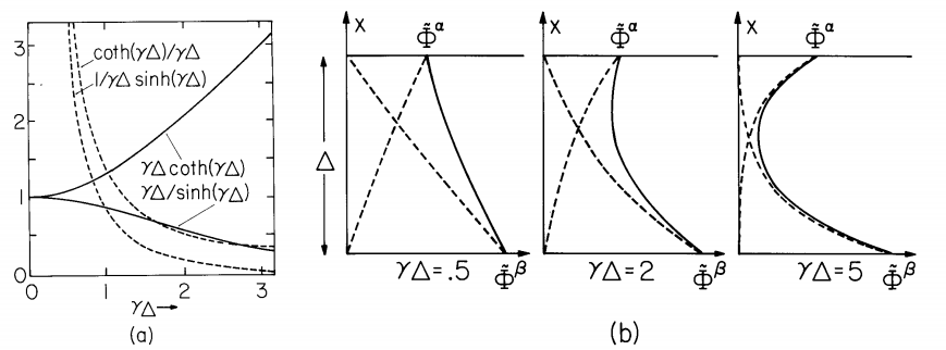
According to Equation (a) of Table 2.16.1, \(D_x\) is induced by a "self term" (proportional to the potential at the same surface) and a "mutual term." The coefficients which express this self- and mutual-coupling have a dependence on \(\Delta \gamma\) (\(2 \pi /\gamma\) the wavelength in the y-z plane) shown in Figure 2.16.1a. Written in the of Equation \ref{15}, the potential has components, excited at each surface, that decay to zero, as shown in Figure 2.16.1b, at a rate that is proportional to how rapidly the fields vary in the y-z plane. For long waves the decay is relatively slow, as depicted by the case \(\Delta \gamma = 0.5\), and the mutual-field is almost as great as the self field. But as the wavelength is shortened relative to \(\Delta (\Delta \gamma \) increased ), the surfaces couple less and less.

In this discussion it is assumed that \(\gamma\) is real, which it is if \(k_y\) and \(k_z\) are real. In fact, the transfer relations are valid and useful for complex values of \((k_y,k_z)\). If these numbers are purely imaginary, the field distributions over the layer cross section are periodic. Such solutions are needed to satisfy boundary conditions imposed in an x-y plane.

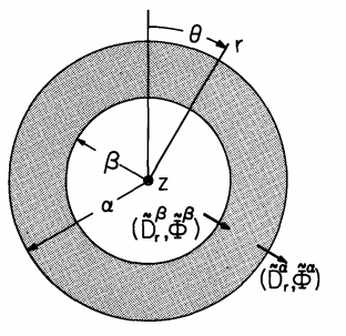
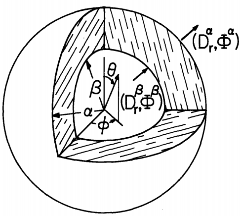
Cylindrical Annulus: With the bounding surfaces coaxial cylinders having radii \(\alpha\) and \(\beta\), it is natural to use cylindrical coordinates \((r, \theta, z)\). A cross section of this prototype region and the coordinates are shown in Table 2.16.2. On the outer and inner surfaces, the potential has the respective forms

\[ \phi(\alpha, \theta, z,t) = Re \tilde{\phi}^{\alpha} (t) e^{-j(m \theta + kz)}; \quad \phi(\beta, \theta,z,t) = Re \tilde{\phi}^{\beta} (t) e^{-j(m \theta + kz)} \label{17} \]

Hence, it is appropriate to assume a bulk potential

\[ \phi = Re \tilde{\phi}(r,t) e^{-j(m \theta + kz)} \label{18} \]

Substitution in Laplace's equation (see Appendix A for operations in cylinderical coordinates), Equation \ref{4}, then shows that

\[ \frac{d^2 \tilde{\phi}}{dr^2} + \frac{1}{r} \frac{d \tilde{\phi}}{dr} - (k^2 + \frac{m^2}{r^2}) \tilde{\phi} = 0 \label{19} \]

Table 2.16.2. Flux-potential relations for cylindrical annulus in terms of electric potential and normal displacement \((\phi, D_r)\). To obtain magnetic relations, substitute \((\phi,D_r, \varepsilon) \rightarrow (\psi,B_r, \mu)\).

	\[ \phi = Re \tilde{\phi} (r,t) e^{-j (m \theta + kz)} \nonumber \]
\[\begin{bmatrix} \tilde{D}_r^{\alpha}\\ \tilde{D}_r^{\beta} \end{bmatrix} = \varepsilon \begin{bmatrix} f_m(\beta,\alpha) & g_m(\alpha,\beta) \\ g_m(\beta,\alpha) & f_m(\alpha,\beta) \end{bmatrix} \begin{bmatrix} \tilde{\phi}^{\alpha}\\ \tilde{\phi}^{\beta} \end{bmatrix} \tag{a} \] \(\underline{k = 0, m = 0}\) \[ f_o (x,y) = \frac{1}{y}/ln(\frac{x}{y}); \quad g_o(x,y) = \frac{1}{x}/ln(\frac{x}{y}) \nonumber \] \(\underline{k = 0, m = 1,2,...}\) \[ f_m(x,y) = \frac{m}{y} \frac{[(\frac{x}{y})^m + (\frac{y}{x})^m]}{[(\frac{x}{y})^m - (\frac{y}{x})^m]} \nonumber \] \[ g_m(x,y) = \frac{2m}{x} \frac{1}{[(\frac{x}{y})^m - (\frac{y}{x})^m]} \nonumber \] \(\underline{k \neq 0, m = 1,2,...^{*}}\) \[ f_m(x,y) = \frac{jk [H_m (jkx) J_m^{'} (jky) - J_m (jkx) H_m^{'} (jky)]}{[J_m (jkx) H_m (jky) - J_m (jky) H_m(jkx)]} \nonumber \] \[ g_m(x,y) = \frac{-2j}{\pi x [J_m (jkx) H_m(jky) - J_m (jky) H_m (jkx)]} \nonumber \] \[ f_m(x,y) = \frac{k [K_m (kx) I_m^{'} (ky) - I_m (kx) K_m^{'} (ky)]}{[I_m (kx) K_m (ky) - I_m (ky) K_m(kx)]} \nonumber \] \[ g_m(x,y) = \frac{1}{x[I_m (kx) K_m (ky) - I_m (ky) K_m(kx)]} \nonumber \]	\[\begin{bmatrix} \tilde{\phi}^{\alpha}\\ \tilde{\phi}^{\beta} \end{bmatrix} = \frac{1}{\varepsilon} \begin{bmatrix} F_m(\beta,\alpha) & G_m(\alpha,\beta) \\ G_m(\beta,\alpha) & F_m(\alpha,\beta) \end{bmatrix} \begin{bmatrix} \tilde{D}_r^{\alpha}\\ \tilde{D}_r^{\beta} \end{bmatrix} \tag{b} \] \(\underline{k = 0, m = 0}\) \[\text{No Inverse} \nonumber \] \(\underline{k = 0, m = 1,2,...}\) \[ F_m(x,y) = \frac{y}{m} \frac{[(\frac{x}{y})^m + (\frac{y}{x})^m]}{[(\frac{x}{y})^m - (\frac{y}{x})^m]} \nonumber \] \[ G_m(x,y) = \frac{2y}{m} \frac{1}{[(\frac{x}{y})^m - (\frac{y}{x})^m]} \nonumber \] \(\underline{k \neq 0, m = 1,2,...^{*}}\) \[ F_m(x,y) = \frac{1}{jk} \frac{[J_m^{'} (jkx) H_m (jky) - H_m^{'} (jkx) J_m (jky) ]}{[J_m^{'} (jky) H_m^{'} (jkx) - J_m^{'} (jkx) H_m^{'}(jky)]} \nonumber \] \[ G_m(x,y) = \frac{-2}{j \pi k (kx) [J_m^{'} (jky) H_m^{'} (jkx) - J_m^{'} (jkx) H_m^{'}(jky)]} \nonumber \] \[ F_m(x,y) = \frac{1}{k} \frac{[I_m^{'} (kx) K_m (ky) - K_m^{'} (kx) I_m (ky) ]}{[I_m^{'} (ky) K_m^{'} (kx) - I_m^{'} (kx) K_m^{'}(ky)]} \nonumber \] \[ G_m(x,y) = \frac{1}{k (kx) [I_m^{'} (ky) K_m^{'} (kx) - I_m^{'} (kx) K_m^{'}(ky)]} \nonumber \]
	\[ \tilde{D}_r^{\alpha} = \varepsilon f_m (0,\alpha) \tilde{\phi}^{\alpha}; \quad f_m(0,\alpha) = - \frac{k I_m^{'} (k \alpha)}{I_m (k \alpha)} \tag{c} \] \[ \tilde{D}_r^{\beta} = \varepsilon f_m (\infty,\beta) \tilde{\phi}^{\beta}; \quad f_m(\infty,\beta) = - \frac{k K_m^{'} (k \beta)}{K_m (k \beta)} \tag{d} \]
* See Prob. 2.17.2 for proof that \(H_m (jkx) J_m^{'} (jkx) - J_m (jkx)H_m^{'} (jkx) = 2/(\pi k x)\) and \(K_m (kx) I_m^{'} (kx) - I_m (kx) K_m^{'} (kx) = 1/kx\) incorporated into \(g_m\) and \(G_m\).

Figure 2.16.2. (a) Modified Bessel functions. (b) Self-field coefficients of cylindrical transfer relations in limits where surfaces do not interact.

By contrast with Equation \ref{13}, this one has space-varying coefficients. It is convenient to categorize the solutions according to the values of \((m,k)\). With \(m = 0\) and \(k = 0\), the remaining terms are a perfect differential which can be integrated twice to give the solutions familiar from the problem of the field between coaxial circular conductors. In view of the boundary conditions at \(r = \alpha\) and \(r = \beta\)

\[ \tilde{\phi} = \tilde{\phi}^{\alpha} \frac{ ln\, (\frac{r}{\beta})}{ ln\, (\frac{\alpha}{\beta})} - \tilde{\phi}^{\beta} \frac{ ln\, (\frac{r}{\alpha})}{ ln\, (\frac{\alpha}{\beta})} = \tilde{\phi}_{\alpha} + ( \tilde{\phi}_{\beta} - \tilde{\phi}_{\alpha}) \frac{ ln\, (\frac{r}{\alpha})}{ ln\, (\frac{\beta}{\alpha})}; \quad (m,k) = (0,0) \label{20} \]

For situations that depend on \(\theta\), but not on \(z\) (polar coordinates) so that \(k = 0\), substitution shows the solutions to Equation \ref{19} are \(r^{\pm m}\). By inspection or algebraic manipulation, the linear combination of these that satisfies the conditions of Equation \ref{17} is

\[ \tilde{\phi} = \tilde{\phi}^{\alpha} \frac{[(\frac{\beta}{r})^m - (\frac{r}{\beta})^m]}{[(\frac{\beta}{\alpha})^m - (\frac{\alpha}{\beta})^m]} + \tilde{\phi}^{\beta} \frac{[(\frac{r}{\alpha})^m - (\frac{\alpha}{r})^m]}{[(\frac{\beta}{\alpha})^m - (\frac{\alpha}{\beta})^m]} ; \quad (m,k) = (m,0) \label{21} \]

For k finite, the solutions to Equation \ref{19} are the modified Bessel functions \(I_m(kr)\) and \(K_m(kr)\). These playa role in the circular geometry analogous to \(exp(\pm\gamma x)\) in Cartesian geometry. The radial dependences of the functions of order \(m = 0\) and \(m = 1\) are shown in Figure 2.16.2a. Note that \(I_m\) and \(K_m\) are respectively singular at infinity and the origin.

Just as the exponential solutions could be determined from Equation \ref{13} by assuming a power series in x, the Bessel functions are determined from an infinite series solution to Equation \ref{19}. Like \(\gamma\), \(k\) can in be complex. If it is, it is customary to define two new functions which, in the special case where \(k\) is real, have imaginary arguments:

\[ J_m (jkr) \equiv j^m I_m (kr), \quad H_m (jkr) = \frac{2}{\pi} j^{-(m+1)} K_m (kr) \label{22} \]

These are respectively the Bessel and Hankel functions of first kind. For real arguments, \(I_m\) and \(K_m\) are real, and hence \(J_m\) and \(H_m\) can be either purely real or imaginary, depending on the order.

Large real-argument limits of the functions \(I_m\) and \(K_m\) reinforce the analogy to the Cartesian exponential solutions:

\[ \lim_{u \to \infty} I_m (u) = \frac{1}{\sqrt{2 \pi u }} exp (u); \quad \lim_{u \to \infty} K_m (u) = \sqrt{\frac{\pi}{2 u}} exp (-u) \label{23} \]

Useful relations in the opposite extreme of small arguments are

\[ \begin{align} &\lim_{u \to 0} jH_o(ju) = \frac{2}{\pi} ln (\frac{2}{1.781072 u}); \quad \lim_{u \to 0} J_m (ju) = \frac{(ju)^m}{m! 2^m} \nonumber \\ \nonumber \\ &\lim_{u \to 0} H_m(ju) = \frac{(m-1)! 2^m}{j \pi (ju)^m} ; \quad m \neq 0 \nonumber \end{align} \label{24} \]

By inspection or algebraic manipulation, the linear combination of \(J_m\) and \(H_m\) satisfying the boundary conditions of Equation \ref{17} is

\[ \tilde{\phi} = \tilde{\phi}^{\alpha} \frac{[ H_m (jk \beta) J_m (jkr) - J_m (jk \beta) H_m (jkr)]}{[ H_m (jk \beta) J_m (jk \alpha) - J_m (jk \beta) H_m (jk \alpha)]} + \tilde{\phi}^{\beta} \frac{[ J_m (jk \alpha) H_m (jkr) - H_m (jk \alpha) J_m (jkr)]}{[ J_m (jk \alpha) H_m (jk \beta) - H_m (jk \alpha) J_m (jk \beta)]} \label{25} \]

The evaluation of the surface displacements \((D_r^{\alpha},D_r^{\beta})\) using Eqs. \ref{20}, \ref{21}, or \ref{25} is now accomplished using the same steps as for the planar layer. The resulting transfer relations are summarized by Equation (a) in Table 2.16.2. Inversion of these relations, to give the surface potentials as functions of the surface displacements, results in the relations summarized by Equation (b) of that table. Primes denote derivatives with respect to the entire specified argument of the function. Useful identities are:

\[ \begin{align} &uI_m^{'} (u) = m I_m (u) + u I_{m+1} (u); \quad u I_m^{'} (u) = -m I_m (u) + u I_{m-1} (u) \nonumber \\ &uK_m^{'} (u) = mK_m (u) - u K_{m+1} (u) \nonumber \\ &R_o^{'} (u) = - R_1 (u) \nonumber \\ &uR_m^{'} (u) = -mR_m(u) + uR_{m-1} (u); \quad uR_m^{'} (u) = mR_m (u) - u R_{m+1} (u) \nonumber \end{align} \label{26} \]

where \(R_m\) can be \(J_m\), \(H_m\), or the function \(N_m\) to be defined with Equation \ref{29}.

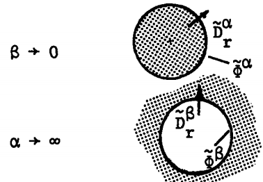
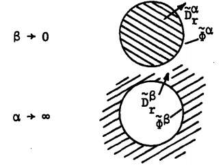
Two useful limits of the transfer relations are given by Eqs. (c) and (d) of Table 2.16.2. In the first, the inner surface is absent, while in the second the outer surface is removed many wavelengths \(2 \pi/k\). The self-field coefficients \(f_m(0,\alpha)\) and \(f_m(\infty,\beta)\) are sketched for \(m=0\) and \(m=1\) in Figure 2.16.2b. Again, it is useful to note the analogy to the planar layer case where the appropriate limit is \(k \Delta \rightarrow \infty\). In fact, for \(k \alpha\) or \(k \beta\) reasonably large, the \(k\) dependence and the signs are the same as for the planar geometry:

\[ \lim_{k \alpha \to \infty} \alpha f_m (0, \alpha) \rightarrow -k \alpha; \quad \lim_{k \beta \to \infty} \beta f_m (\infty, \beta) \rightarrow k \beta \label{27} \]

For small arguments, these functions become

\[ \begin{align} &\lim_{k \alpha \to 0} \alpha f_o (0, \alpha) \rightarrow - \frac{(k \alpha)^2}{2}; \quad \lim_{k \beta \to 0} \beta f_o (\infty, \beta) \rightarrow \frac{1}{ln [\frac{2}{1.781072 k \beta}]} \nonumber \\ &\lim_{k \alpha \to 0} \alpha f_m(0,\alpha) \rightarrow -m\, for\, m \neq 0; \quad \lim_{k \beta \to 0} \beta f_m(\infty,\beta) \rightarrow m\, for\, m \neq 0 \nonumber \end{align} \label{28} \]

In general, \(k\) can be complex. In fact the most familiar form for Bessel functions is with \(k\) purely imaginary. In that case, \(J_m\) is real but \(H_m\) is complex. By convention

\[ H_m (u) \equiv J_m (u) + j N_m (u) \label{29} \]

where, if \(u\) is real, Jm and Nm are real and Bessel functions of first and second kind. As might be expected from the planar analogue, the radial dependence becomes periodic if \(k\) is imaginary. Plots of the functions in this case are given in Figure 2.16.3.

Figure 2.16.3. Bessel functions of first and second kind and real arguments. References for the Bessel and related functions should be consulted for more details concerning their properties and numerical values.\(^{1-4}\)

Spherical Shell: A region between spherical surfaces having outer and inner radii \(\alpha\) and \(\beta\), respectively, is shown in the figure of Table 2.16.3. In the volume, the potential conveniently takes the variable separable form

\[ \phi = Re \tilde{\phi} (r,t) \quad \Theta (\theta) e^{-j m \phi} \label{30} \]

where \((r, \theta, \phi)\) are spherical coordinates as defined in the figure. Substitution of Equation \ref{30} into Laplace equation, Equation \ref{4}, shows that the \(\phi\) dependence is correctly assumed and that the \((r,\theta)\) dependence is determined from the equations

\[ \begin{align} &\frac{1}{sin\, \theta \Theta} \frac{d}{d \theta} [ sin\, \theta \frac{d \Theta}{ d\theta}] - \frac{m^2}{sin^2 \, \theta} = -K^2 \nonumber \\ \nonumber \\ &\frac{1}{\tilde{\phi}} \frac{d}{dr} (r^2 \frac{d \tilde{\phi}}{dr}) = K^2 \nonumber \end{align} \label{31} \]

where the separation coefficient \(K^2\) is independent of \((r,\theta)\). With the substitutions

\[ u = cos\, \theta, \, \sqrt{1 - u^2} = sin \, \theta \label{32} \]

Equation \ref{31} (a) is converted to

\[ (1-u^2) \frac{d^2 \Theta}{du^2} - 2u \frac{d\Theta}{du} + (K^2 - \frac{m^2}{1-u^2})\, \Theta = 0 \label{33} \]

For \(K^2 = n(n+1)\) and \(n\) an integer, solutions to Equation \ref{33} are

\[ \Theta = P_n^M (u) \label{34} \]

Table 2.16.3. Flux-potential transfer relations for spherical in terms of electric potential and normal displacement \((\phi,D_r)\). To obtain magnetic relations, substitute \((\phi, D_r, \varepsilon) \rightarrow (\psi, B_r, \mu)\).

				\[ \begin{align} &\phi = Re \tilde{\phi} (r,t) P_n^m (cos \, \theta) e^{-jm \phi} \nonumber \\ &P_n^m = (1- x^2)^{m/2} \frac{d^m P_n}{dx^m} \nonumber \\ &P_o = 1, \quad P_1 = x, \quad P_2 = \frac{1}{2} (3 x^2 -1) \nonumber \\ &P_3 = \frac{1}{2} (5x^3 - 3x) \nonumber \\ &P_4 = \frac{1}{8} (35x^4 - 30x^2 +3) \nonumber \end{align} \nonumber \]
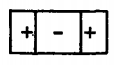
\(m\)	\(P_o^m\)	\(P_1^m\)	\(P_1^m cos \, m \phi\)	\(P_2^m\)	\(P_2^m cos \, m \phi\)	\(P_3^m\)	\( P_3^m cos \, m \phi\)
\(0\)	\(1\)	\( cos \, \theta\)		\(\frac{1}{2} (3 cos^2 \, \theta -1)\)		\(\frac{1}{2} (5 cos^3 \, \theta - 3 cos \, \theta)\)
\(1\)	\(0\)	\( sin \, \theta\)		\( 3 sin \, \theta cos \, \theta\)		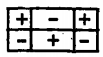\(\frac{3}{2} sin \, \theta (5 cos^2 \, \theta -1) \)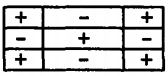
\(2\)	\(0\)	\(0\)		\(3 sin^2 \, \theta\)\)		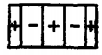\(15 sin^2 \, \theta cos \, \theta \)
\(3\)	\(0\)	\(0\)		\(0\)		\(15 sin^3\, \theta \)
\[\begin{bmatrix} \tilde{D}_r^{\alpha}\\ \tilde{D}_r^{\beta} \end{bmatrix} = \varepsilon \begin{bmatrix} f_n(\beta,\alpha) & g_n(\alpha,\beta) \\ g_n(\beta,\alpha) & f_n(\alpha,\beta) \end{bmatrix} \begin{bmatrix} \tilde{\phi}^{\alpha}\\ \tilde{\phi}^{\beta} \end{bmatrix} \tag{a} \] \[ f_n(x,y) = \frac{[n(\frac{y}{x})^n + (n+1) (\frac{x}{y})^{n+1}]}{[x(\frac{x}{y})^n - y(\frac{y}{x})^n]} \nonumber \] \[ g_n(x,y) = \frac{(2n +1)}{x^2 [ \frac{1}{y} (\frac{x}{y})^n - \frac{1}{x}(\frac{y}{x})^n]} \nonumber \]				\[\begin{bmatrix} \tilde{\phi}^{\alpha}\\ \tilde{\phi}^{\beta} \end{bmatrix} = \frac{1}{\varepsilon} \begin{bmatrix} F_n(\beta,\alpha) & G_n(\alpha,\beta) \\ G_n(\beta,\alpha) & F_n(\alpha,\beta) \end{bmatrix} \begin{bmatrix} \tilde{D}_r^{\alpha}\\ \tilde{D}_r^{\beta} \end{bmatrix} \tag{b} \] \[ F_n(x,y) = \frac{y}{x} \frac{[\frac{1}{n} (\frac{y}{x})^n + \frac{1}{n+1} (\frac{x}{y})^{n+1} ]} {[\frac{1}{y} (\frac{x}{y})^n - \frac{1}{x} (\frac{y}{x})^n]} \nonumber \] \[ G_n(x,y) = \frac{y}{x} \frac{(2n+1)}{n(n+1)} \frac{1} {[\frac{1}{y} (\frac{x}{y})^n - \frac{1}{x} (\frac{y}{x})^n]} \nonumber \]
				\[ \tilde{D}_r^{\alpha} = - \frac{\varepsilon n}{\alpha} \tilde{\phi} ^{\alpha} \tag{c} \] \[\tilde{D}_r^{\beta} = - \frac{\varepsilon (n+1)}{\beta} \tilde{\phi} ^{\beta} \tag{d} \]

where \(P_m\) are the associated Legendre functions of the first kind, order n and degree m. In terms of the Legendre polynomials \(P_n\), these functions are summarized in Table 2.16.3. Note that these solutions are closed. They do not require infinite series for their representation.

To the second order differential equation, Equation \ref{33}, there must be a second set of solutions \(Q_n^m\). Because these are singular in the interval \(0 \leqslant \theta \leqslant \pi\), and situations of interest here include the entire spherical surface at any given radius, these solutions are not included. The functions \(P_n^m\) play the role of \(exp(jkz)(say)\) in cylindrical geometry, while \(exp(jm \phi)\) is analogous to exp(jm \theta). The radial dependence, which is much of the bother in cylindrical coordinates, is actually quite simple in spherical coordinates. From Equation \ref{31} b it is seen that solutions are a linear combination of \(r^n\) and \(r^{-(n+1)}\). With the assumption that surface potentials respectively have the form

\[ \phi ({\alpha \atop \beta}, \theta, \phi, t) = Re \tilde{\phi}^{\alpha \atop \beta} (t) P_n^m (cos\, \theta)\, exp(jm \phi) \label{35} \]

The complex amplitudes \((\tilde{\phi}^{\alpha},\tilde{\phi}^{\beta})\) determine the combination of \(cos\, m \phi\) and \(sin\, m \phi\), constituting the distribution of \(\phi\) with longitudinal distance. For a real amplitude, the distribution is proportional to cos mý. In the summary of Table 2.16.3, the lowest orders of \( P_n^m \, (cos\, m \phi)\) are tabulated, together with diagrams showing the zones that are positive and negative relative to each other. In the rectangular plots, the ordinate is \(0 \leqslant \theta \leqslant \pi\), while the abscissa is \(0 \leqslant \phi \leqslant 2 \pi\). Thus, the top and bottom lines are the north and south poles while the lines within are nodes. The horizontal register of each diagram is determined by the complex amplitude, which determines the phase of \(exp(jm \phi)\).

Evaluation of the transfer relations given in Table 2.16.3 by Eqs. (a) and (b) is now carried out following the same procedure as for the planar layer. From these relations follow the limiting situations of a solid spherical region or one where the outer surface is well removed from the region of interest summarized for reference by Eqs. (c) and (d) of Table 2.16.3.

Further useful aspects of solutions to Laplace's equation in spherical coordinates, including orthogonality relations that permit Fourier-like expansions and evaluation of averages, are given in standard references.\(^5\)

---

1. F. B. Hildebrand, Advanced Calculus for Applications, Prentice-Hall, Englewood Cliffs, N.J., 1962 pp. 142-165.

2. S. Ramo, J. R. Whinnery and T. Van Duzer, Fields and Waves in Communication Electronics, John Wil and Sons, New York, 1965, pp. 207-218.

3. M. Abramowitz and I. A. Stegun, Handbook of Mathematical Functions with Formulas, Graphs, and Mat matical Tables, National Bureau of Standards, Applied Mathematics Series 55, U.S. Government Prin Office, Washington D. C. 20402, 1964, pp. 355-494.

4. E. Jahnke and F. Emde, Table of Functions with Formulae and Curves, Dover Publications, New York. 1945, pp. 128-210

5. F. B. Hildebrand, loc. cit., pp. 159-165.