
3.6: Polarization and Magnetization Force Densities on Tenuous Dipoles
- Page ID
- 28136

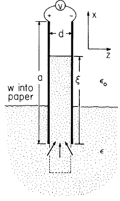
Forces due to polarization and magnetization lend further emphasis to the importance of making a distinction between forces on microscopic charged particles and macroscopic forces on materials sup-porting those charges. The experiment depicted by Figure 3.6.1 makes it clear that (1) there is more to the force density than accounted for by the Lorentz force density, and (2) the additional force density is not \(\rho_p \overrightarrow{E}\) (or in the magnetic analogue, \(\rho_m \overrightarrow{H}\)).
A pair of capacitor plates are dipped into a dielectric liquid. With the application of a potential difference \(v\), it is found experimentally that the liquid rises between the plates.* To make it clear that the issues involved can be understood in terms of lumped-parameter concepts, the liquid between the plates is replaced by a solid dielectric material having the same polarizability as the liquid, so that the-z- problem is reduced to one of a solid dielectric slab rising between the plates as it is pulled from the liquid below.
Recall that if the interface is well removed from thew into edges of the plates, an exact solution satisfying the quasi-paperstatic differential equations and boundary conditions in the neighborhood of the interface is \( \overrightarrow{E} = (v/d) \overrightarrow{i}_z\). Of course,there is a fringing field in the neighborhood of the edges of the capacitor plates. However, because the slab and the liquid have the same dielectric constant and \(p_f = 0\), the fringing field has the same distribution as if the dielectric were not present.
It might be tempting to take the force as being the product of the net charge at any given point and the local electric field, or \(\rho_p \overrightarrow{E}\). However, everywhere in the dielectric bulk the polarization density is proportional by the same constant to the electric field (Equation 2.16.1). Because \(\rho_f = 0\), it follows from Gauss' law that \(\overrightarrow{E}\) and hence \(\overrightarrow{P}\) have no divergence, and so there is also no polarization charge in the dielectric. Furthermore, because the electric field is uniform and tangential to the interface, there is not even a polarization surface charge density at the interface(Equation 2.10.21). Throughout the dielectric, on the interface and in the bulk, there is no polarization charge. Clearly, the force which makes the dielectric rise between the plates cannot be accounted for by a polarization charge density.
If the polarized material is composed of individual dipoles, each subject to an electrical force, and each transmitting this electrical force to the neutral medium, it is clear that there is really no reason to expect that the force density should take the same form as that for free charges. With free charges, it is the individual charges that transmit their forces to the neutral medium through mechanisms discussed in Sec. 3.2. Now concern is with the force on individual dipoles which transmit that force to the neutral medium, either because they are tied to a lattice structure (Figure 2.8.1) or through collisional mechanisms similar to those discussed for charge carriers in Sec. 3.2.
In the following. it is assumed that the dipoles are subject to an electric field that is the average, or macroscopic, electric field. The development ignores the distortion of the electric field intensity at one dipole because of the neighboring dipoles. For this reason, the result is designated a force density acting on tenuous dipoles.

A single dipole is shown in Figure 3.6.2. The dipole can be pictured as a pair of oppositely signed charges having the vector separation \(\overrightarrow{d}\). The negative charge is located at \(\overrightarrow{r}\). With the assumption that the force on the dipole is transmitted to the medium, the procedure is to compute the force on a single dipole, and then to average this force over all the dipoles. The net force in the ith direction on the pair of charges taken as a unit is
\[ f_i = \lim_{\overrightarrow{d} \to 0 \\ q \to \infty} q \big [ E_i (\overrightarrow{r} + \overrightarrow{d}) - E_i (\overrightarrow{r}) \big] \label{2} \]
The limit is one in which the spacing of the charges becomes extremely small compared to other distances of interest and, at the same time, the magnitude of the charges becomes very large, so that the product \(q \overrightarrow{d} \equiv \overrightarrow{p}\) remains finite. The dipole moment is defined as \(\overrightarrow{p}\) The required limit of Equation \ref{2} becomes
\[ f_i = \lim_{\overrightarrow{d} \to 0 \\ q \to \infty} q \big [ E_i (\overrightarrow{r}) + \frac{\partial{E_i}}{\partial{x_j}} d_j - E_i (\overrightarrow{r}) \big ] = P_j \frac{\partial{E_i}}{\partial{x_j}} \label{3} \]
Thus, there is a net force on each dipole given in vector notation by
\[ \overrightarrow{f} = \overrightarrow{p} \cdot \nabla \overrightarrow{E} \label{4} \]
Note that implicit to this vector representation is the definition of what is meant by the operator \(\overrightarrow{A} \cdot \nabla \overrightarrow{B} \)
By assumption, the net force on each dipole is transmitted to the macroscopic medium and it is appropriate then to think of averaging these polarization forces over all dipoles within the medium.In general, this average would have to be taken with recognition that the microscopic dipoles could assume a spectrum of polarizations in a given electric field intensity. For present purposes, the average can simply be represented as the multiplication of Equation \ref{4} by the number of dipoles, \(n\), per unit volume. With the definition of the polarization density as \(\overrightarrow{P} = n \overrightarrow{p} \), the Kelvin polarization force density is found:
\[ \overrightarrow{F} = \overrightarrow{P} \cdot \nabla \overrightarrow{E} \label{5} \]
Can the force density given by Equation \ref{5} be used to explain the rise of the dielectric between the plates in Figure 3.6.1? Certainly, there is no force density in material regions of uniform electric field, because then the -spatial derivatives called for with Equation \ref{5} vanish. However, in the fringing field at the lower edges of the plates, the electric field intensity does vary rapidly. In that region,the permittivity is a constant, and for a linear dielectric, where \(\overrightarrow{D} = \varepsilon \overrightarrow{E}\), Equation \ref{5} becomes [in dealing with vectors and tensors, a term in which a subscript appears twice is to be summed 1 to 3 (unless otherwise indicated)]
\[ F_i = (\varepsilon - \varepsilon_o) E_j \frac{\partial{E_i}}{\partial{x_j}} = (\varepsilon - \varepsilon_o) E_j \frac{\partial{E_j}}{\partial{x_i}} = (\varepsilon - \varepsilon_o) \frac{\partial{}}{\partial{x_i}} (\frac{1}{2} E_j E_j) \label{6} \]
where the irrotational nature of \(\overrightarrow{E}\) is exploited, \(\partial{E_i}/\partial{x_j} = \partial{E_j}/ \partial{x_i}\). In vector notation, Equation \ref{6} becomes
\[ \overrightarrow{F} = \nabla [ \frac{1}{2} (\varepsilon - \varepsilon_o ) \overrightarrow{E} \cdot \overrightarrow{E} ] \label{7} \]
Remember, this relation pertains only to regions of a linear dielectric in which the permittivity is constant, and is simply a means of visualizing the distribution of the Kelvin force density. In such regions, the force density has the direction of maximum rate of increase of the electric energy storage.Typical force vectors, sketched in Figure 3.6.1, tend to push the dielectric upward between the plates. It is important not to over generalize from Equation \ref{7}. In any configuration in which there is a component of \(\overrightarrow{E}\) perpendicular to an interface, there is a singular component of the Kelvin force density acting at the interface -- a surface force density. Such a component would be incorrectly inferred from Equation \ref{7} ,which is not valid through the interfacial region.
Consider now the force density acting on a continuum of dilute magnetic dipoles that, like the analogous electric dipoles just considered, pass along a force of electric origin to a macroscopic medium via collisions or lattice constraints. It is not possible to use the Lorentz force law as a starting point unless magnetic monopoles and an analogous force law on these magnetic "charges" is postulated. Without introducing such notions, the Kelvin magnetization force density can be deduced as follows.
Electroquasistatic and magnetoquasistatic systems are pictured abstractly in Figure 3.6.3. A volume enclosing the region occupied by a dipole having the position \(\overrightarrow{\xi}\) has a surface \(S\) and includes neither free charge in the EQS system nor free current in the MQS system. Hence the fields are governed by
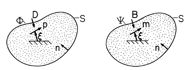
\[ \begin{align} &\nabla \times \overrightarrow{E} = 0 ; \quad \overrightarrow{E} = -\nabla \phi \quad \quad \quad &\nabla \times \overrightarrow{H} = 0; \quad \overrightarrow{H} = -\nabla \psi \label{8} \\ &\nabla \cdot (\varepsilon_o \overrightarrow{E} + \overrightarrow{P}) = 0; \quad \overrightarrow{P} = n \overrightarrow{p} \quad \quad \quad &\nabla \cdot (\mu_o \overrightarrow{H} + \mu_o \overrightarrow{H}) = 0; \quad \overrightarrow{M} = n \overrightarrow{m} \label{9} \end{align} \]
Statements that the input of electric energy either goes into increasing the total energy stored or in-to doing work on the dipoles are (see Eqs. 3.5.1 and 2.13.4 or Eq. 3.5.10 and Eq. 2.14.9 integrated by parts):
\[ \begin{align} &\oint_S \phi \delta \overrightarrow{D} \cdot \overrightarrow{n} da = \delta w + \overrightarrow{f} \cdot \delta \overrightarrow{\xi} \quad \quad \quad &\oint_S \psi \delta \overrightarrow{B} \cdot \overrightarrow{n} da = \delta w + \overrightarrow{f} \cdot \delta \overrightarrow{\xi} \label{10} \end{align} \]
To find the force on the dipole, the energy would be determined as a function of the electrical excitations and \(\xi\). Then, with the understanding that the derivative is taken with the quantities \(\overrightarrow{D} \cdot \overrightarrow{n}\) and \(\overrightarrow{B} \cdot \overrightarrow{n}\), respectively, held fixed on the surface \(S\), the respective forces follow as
\[ \begin{align} &f_i = - \frac{\partial{w}}{\partial{\xi_i}} \quad \quad \quad &f_i = - \frac{\partial{w}}{\partial{\xi_i}} \label{11} \end{align} \]
Now, what would be obtained if this procedure were carried through for the electric case is already known to be given by Equation \ref{4}. Moreover, there is a complete analogy between every aspect of the electric and magnetic systems. The calculation in the magnetic case need not be repeated once the electric one is carried out. Rather, an identification of variables suffices to give the answer, \(\overrightarrow{E} \rightarrow \overrightarrow{H}, \, \overrightarrow{P} \rightarrow \mu_o \overrightarrow{M}\).Hence, it follows that Equation \ref{5} is replaced by the Kelvin magnetization force density
\[ \overrightarrow{F} = \mu_o \overrightarrow{M} \cdot \nabla \overrightarrow{H} \label{12} \]
The Kelvin force densities, Eqs. \ref{5} and \ref{12} , suffer the weakness that they do not take into account the interaction between dipoles. Moreover, is the average over the spectrum of dipole moments \(\overrightarrow{p}\) or \(\overrightarrow{m}\) leading to the polarization and magnetization densities consistent with the usage of these densities in Chapter 2? These difficulties are overcome by a derivation based on thermodynamic principles. Because force densities are then based on electrically measured constitutive laws, consistency with definitions already introduced is insured.
* In an experiment, a-c voltage is used with a sufficiently high frequency that the material responds only to the rms field and free charge cannot accumulate in the bulk.