
14.3: Continuous Symmetries and Infinitesimal Generators
- Page ID
- 19028
\( \newcommand{\vecs}[1]{\overset { \scriptstyle \rightharpoonup} {\mathbf{#1}} } \)
\( \newcommand{\vecd}[1]{\overset{-\!-\!\rightharpoonup}{\vphantom{a}\smash {#1}}} \)
\( \newcommand{\dsum}{\displaystyle\sum\limits} \)
\( \newcommand{\dint}{\displaystyle\int\limits} \)
\( \newcommand{\dlim}{\displaystyle\lim\limits} \)
\( \newcommand{\id}{\mathrm{id}}\) \( \newcommand{\Span}{\mathrm{span}}\)
( \newcommand{\kernel}{\mathrm{null}\,}\) \( \newcommand{\range}{\mathrm{range}\,}\)
\( \newcommand{\RealPart}{\mathrm{Re}}\) \( \newcommand{\ImaginaryPart}{\mathrm{Im}}\)
\( \newcommand{\Argument}{\mathrm{Arg}}\) \( \newcommand{\norm}[1]{\| #1 \|}\)
\( \newcommand{\inner}[2]{\langle #1, #2 \rangle}\)
\( \newcommand{\Span}{\mathrm{span}}\)
\( \newcommand{\id}{\mathrm{id}}\)
\( \newcommand{\Span}{\mathrm{span}}\)
\( \newcommand{\kernel}{\mathrm{null}\,}\)
\( \newcommand{\range}{\mathrm{range}\,}\)
\( \newcommand{\RealPart}{\mathrm{Re}}\)
\( \newcommand{\ImaginaryPart}{\mathrm{Im}}\)
\( \newcommand{\Argument}{\mathrm{Arg}}\)
\( \newcommand{\norm}[1]{\| #1 \|}\)
\( \newcommand{\inner}[2]{\langle #1, #2 \rangle}\)
\( \newcommand{\Span}{\mathrm{span}}\) \( \newcommand{\AA}{\unicode[.8,0]{x212B}}\)
\( \newcommand{\vectorA}[1]{\vec{#1}} % arrow\)
\( \newcommand{\vectorAt}[1]{\vec{\text{#1}}} % arrow\)
\( \newcommand{\vectorB}[1]{\overset { \scriptstyle \rightharpoonup} {\mathbf{#1}} } \)
\( \newcommand{\vectorC}[1]{\textbf{#1}} \)
\( \newcommand{\vectorD}[1]{\overrightarrow{#1}} \)
\( \newcommand{\vectorDt}[1]{\overrightarrow{\text{#1}}} \)
\( \newcommand{\vectE}[1]{\overset{-\!-\!\rightharpoonup}{\vphantom{a}\smash{\mathbf {#1}}}} \)
\( \newcommand{\vecs}[1]{\overset { \scriptstyle \rightharpoonup} {\mathbf{#1}} } \)
\(\newcommand{\longvect}{\overrightarrow}\)
\( \newcommand{\vecd}[1]{\overset{-\!-\!\rightharpoonup}{\vphantom{a}\smash {#1}}} \)
\(\newcommand{\avec}{\mathbf a}\) \(\newcommand{\bvec}{\mathbf b}\) \(\newcommand{\cvec}{\mathbf c}\) \(\newcommand{\dvec}{\mathbf d}\) \(\newcommand{\dtil}{\widetilde{\mathbf d}}\) \(\newcommand{\evec}{\mathbf e}\) \(\newcommand{\fvec}{\mathbf f}\) \(\newcommand{\nvec}{\mathbf n}\) \(\newcommand{\pvec}{\mathbf p}\) \(\newcommand{\qvec}{\mathbf q}\) \(\newcommand{\svec}{\mathbf s}\) \(\newcommand{\tvec}{\mathbf t}\) \(\newcommand{\uvec}{\mathbf u}\) \(\newcommand{\vvec}{\mathbf v}\) \(\newcommand{\wvec}{\mathbf w}\) \(\newcommand{\xvec}{\mathbf x}\) \(\newcommand{\yvec}{\mathbf y}\) \(\newcommand{\zvec}{\mathbf z}\) \(\newcommand{\rvec}{\mathbf r}\) \(\newcommand{\mvec}{\mathbf m}\) \(\newcommand{\zerovec}{\mathbf 0}\) \(\newcommand{\onevec}{\mathbf 1}\) \(\newcommand{\real}{\mathbb R}\) \(\newcommand{\twovec}[2]{\left[\begin{array}{r}#1 \\ #2 \end{array}\right]}\) \(\newcommand{\ctwovec}[2]{\left[\begin{array}{c}#1 \\ #2 \end{array}\right]}\) \(\newcommand{\threevec}[3]{\left[\begin{array}{r}#1 \\ #2 \\ #3 \end{array}\right]}\) \(\newcommand{\cthreevec}[3]{\left[\begin{array}{c}#1 \\ #2 \\ #3 \end{array}\right]}\) \(\newcommand{\fourvec}[4]{\left[\begin{array}{r}#1 \\ #2 \\ #3 \\ #4 \end{array}\right]}\) \(\newcommand{\cfourvec}[4]{\left[\begin{array}{c}#1 \\ #2 \\ #3 \\ #4 \end{array}\right]}\) \(\newcommand{\fivevec}[5]{\left[\begin{array}{r}#1 \\ #2 \\ #3 \\ #4 \\ #5 \\ \end{array}\right]}\) \(\newcommand{\cfivevec}[5]{\left[\begin{array}{c}#1 \\ #2 \\ #3 \\ #4 \\ #5 \\ \end{array}\right]}\) \(\newcommand{\mattwo}[4]{\left[\begin{array}{rr}#1 \amp #2 \\ #3 \amp #4 \\ \end{array}\right]}\) \(\newcommand{\laspan}[1]{\text{Span}\{#1\}}\) \(\newcommand{\bcal}{\cal B}\) \(\newcommand{\ccal}{\cal C}\) \(\newcommand{\scal}{\cal S}\) \(\newcommand{\wcal}{\cal W}\) \(\newcommand{\ecal}{\cal E}\) \(\newcommand{\coords}[2]{\left\{#1\right\}_{#2}}\) \(\newcommand{\gray}[1]{\color{gray}{#1}}\) \(\newcommand{\lgray}[1]{\color{lightgray}{#1}}\) \(\newcommand{\rank}{\operatorname{rank}}\) \(\newcommand{\row}{\text{Row}}\) \(\newcommand{\col}{\text{Col}}\) \(\renewcommand{\row}{\text{Row}}\) \(\newcommand{\nul}{\text{Nul}}\) \(\newcommand{\var}{\text{Var}}\) \(\newcommand{\corr}{\text{corr}}\) \(\newcommand{\len}[1]{\left|#1\right|}\) \(\newcommand{\bbar}{\overline{\bvec}}\) \(\newcommand{\bhat}{\widehat{\bvec}}\) \(\newcommand{\bperp}{\bvec^\perp}\) \(\newcommand{\xhat}{\widehat{\xvec}}\) \(\newcommand{\vhat}{\widehat{\vvec}}\) \(\newcommand{\uhat}{\widehat{\uvec}}\) \(\newcommand{\what}{\widehat{\wvec}}\) \(\newcommand{\Sighat}{\widehat{\Sigma}}\) \(\newcommand{\lt}{<}\) \(\newcommand{\gt}{>}\) \(\newcommand{\amp}{&}\) \(\definecolor{fillinmathshade}{gray}{0.9}\)Definition of Infinitesimal Generator
Symmetry transformations can be described as transformations of the independent and dependent variables. Continuous symmetry transformations can be described as transformations of these variables which depend on a, possibly infinitesimal, parameter ε.
\[t \rightarrow \tilde t= F(\varepsilon)t \nonumber \]
\[y \rightarrow \tilde y= F(\varepsilon)y \nonumber \]
The operator \(F(\varepsilon)\) describes the transformation. It is a function of the infinitesimal parameter \(\varepsilon\), and it may also depend on \(t\) and \(y\). Furthermore, it is an operator meaning that it may involve derivative operations.
We are considering only continuous symmetries, so we can study the behavior in the limit as \(\varepsilon \rightarrow 0\). The operator \(F(\varepsilon)\) can be written as a Taylor series in the small parameter \(\varepsilon\).
\[F(\varepsilon) = 1 + \varepsilon U + \frac{1}{2!}\varepsilon^2U^2 + \ldots \nonumber \]
The term \(U\) in the expansion above is called the infinitesimal generator. It may be separated into two components.
\[U = \xi \partial_t + \eta \partial_y \nonumber \]
The function \(\xi\) describes infinitesimal variation in the independent variable. The function \(\eta\) describes infinitesimal variation in the dependent variable, and it was introduced in Sec. 11.3. Both \(\xi\) and \(\eta\) may depend on both the independent variable and the dependent variable.
\[\xi = \xi (t,y) \nonumber \]
\[\eta = \eta (t,y) \nonumber \]
In the limit of \(\varepsilon \rightarrow 0\), we can ignore terms of order \(\varepsilon^2\) or higher.
\[F(\varepsilon) \approx 1 + \varepsilon U \nonumber \]
An infinitesimal generator describes a continuous symmetry transformation. If we know an infinitesimal generator for some continuous symmetry, we can find the corresponding transformation
\[t \rightarrow e^{\varepsilon U}t \quad \text{ and } \quad y \rightarrow e^{\varepsilon U}y. \label{14.3.8} \]
To understand where this relationship between infinitesimal generators and finite transformations come from, consider the Taylor expansion of \(e^{\varepsilon U}\) [14, p. 33].
\[e^{\varepsilon U} = 1 + \epsilon U + \frac{1}{2!}(\varepsilon U)^2 + \frac{1}{3!}(\varepsilon U)^3 + \ldots \nonumber \]
In the limit as \(\varepsilon \rightarrow 0\),
\[e^{\varepsilon U} \approx 1 + \varepsilon U. \nonumber \]
Therefore, the corresponding infinitesimal transformation for \(\varepsilon \rightarrow 0\) is given by
\[t \rightarrow t (1+\varepsilon \xi) \nonumber \]
\[y \rightarrow y (1+\varepsilon \eta). \nonumber \]
Infinitesimal Generators of the Wave Equation
As an example, consider infinitesimal generators of the wave equation
\[\frac{d^2y}{dt^2} + \omega_0^2y = 0 \label{14.3.13} \]
As mentioned above, the wave equation contains a continuous symmetry of the form \(t \rightarrow t + \varepsilon\). This continuous symmetry transformation has the form
\[t \rightarrow t(1+\varepsilon \xi) \quad \text { and } \quad y \rightarrow y(1+\varepsilon \eta) \nonumber \]
with \(\xi = 1\) and \(\eta = 0\). It can be described by the infinitesimal generator
\[U = \xi \partial_t + \eta \partial_y = \partial_t. \nonumber \]
More generally, infinitesimal generators and finite transformations are related by Equation \ref{14.3.8}, so finite transformations can be derived from infinitesimal generators.
\[t \rightarrow \left(e^{\varepsilon \partial_t}\right) t = \left(1+\varepsilon \partial_{t}+\frac{1}{2 !} \left(\varepsilon \partial_{t}\right)^{2}+ \ldots \right) t = t+\varepsilon \nonumber \]
\[y \rightarrow \left(e^{\varepsilon \partial_t}\right) y = \left(1+\varepsilon \partial_{t}+\frac{1}{2 !} \left(\varepsilon \partial_{t}\right)^{2}+ \ldots \right) y = y. \nonumber \]
While the symmetry transformation was given in this example, below we will see a procedure to derive infinitesimal generators for an equation.
In general, if we know a solution to an equation and we know that a symmetry is present, we can derive a whole family of related solutions to the equation without having to go through the work of solving the equation again. The wave equation, Equation \ref{14.3.13}, has solutions of the form
\[y(t) = c_0 \cos (\omega_0t) + c_1 \sin (\omega_0t) \label{14.3.18} \]
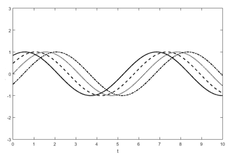
where boundary conditions determine the constants \(c_0\) and \(c_1\). The symmetry described by the infinitesimal generator \(U = \partial t\) tells us that
\[y(t) = c_0 \cos (\omega_0(t+ \varepsilon)) + c_1 \sin (\omega_0 (t+ \varepsilon)) \label{14.3.19} \]
must also be a solution. Using Equation \ref{14.3.18}, we have found a family of related solutions because Equation \ref{14.3.19} is a solution for all finite or infinitesimal constants \(\varepsilon\). Figure \(\PageIndex{1}\) illustrates this idea. The known solution is shown as a solid line. The dotted and dashed lines illustrate related solutions, for different constant \(\varepsilon\) values. We encountered the wave equation in the mass spring example of Section 11.4 and the capacitor inductor example of Section 11.5, so symmetry analysis provides information about both of these energy conversion processes. It tells us that if we run the energy conversion process and find one physical path \(y(t)\), then for appropriate boundary conditions, \(y(t + \varepsilon)\) is also a physical path. This symmetry is present in all time invariant systems. Qualitatively for the mass spring example, it tells us that if we know the path taken by the mass when we remove the restraint today, then we know the path taken by the mass when we repeat the experiment tomorrow , and we know this idea from symmetry analysis without having to re-analyze the system.
All linear equations, including the wave equation, contain a continuous symmetry transformation described by the infinitesimal generator
\[U = y\partial_y \nonumber \]
which corresponds to \(\xi = 0\) and \(\eta = y\). Again, we can find the corresponding finite transformation using Equation \ref{14.3.8}.
\[t \rightarrow \left(e^{\varepsilon y \partial_y}\right) t = \left(1+\varepsilon y \partial_{y} +\frac{1}{2 !} \left(\varepsilon y \partial_{y}\right)^{2} + \ldots \right) t = t \nonumber \]
and
\[y \rightarrow \left(e^{\varepsilon y \partial_y}\right) y = \left(1+\varepsilon y \partial_{y} +\frac{1}{2 !} \left(\varepsilon y \partial_{y}\right)^{2}+ \ldots \right) y = y(1+ \varepsilon). \nonumber \]
To summarize this transformation,
\[t \rightarrow t \nonumber \]
and
\[y \rightarrow y(1 + \varepsilon) \nonumber \]
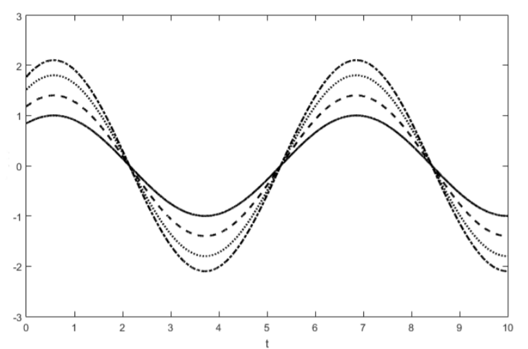
The above transformation says that if we scale any solution of a linear equation, \(y(t)\), by a constant \((1 + \varepsilon)\), the result will also be a solution of the equation. By definition, a linear equation obeys exactly this property. By knowing a solution of the wave equation and this symmetry, we can find a whole family of related solutions, and this family of solutions is illustrated in Figure \(\PageIndex{2}\).
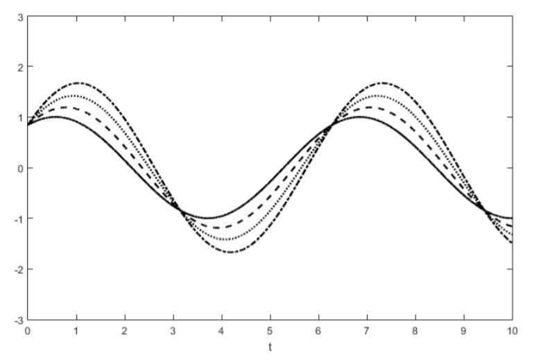
The wave equation also contains the symmetry transformation described by the infinitesimal generator
\[U = \sin (\omega_0t) \partial_y. \nonumber \]
The operators ξ and η can be identified directly from the infinitesimal generator.
\[\xi = 0 \nonumber \]
\[\eta = \sin (\omega_0t) \nonumber \]
Again we can find the corresponding finite transformations using Equation 14.3.8.
\[t \rightarrow e^{\varepsilon U}t =t \nonumber \]
\[y \rightarrow e^{\varepsilon U} y = \left(1+\varepsilon \sin (\omega_0t) \partial_{y} +\frac{1}{2 !} \left(\varepsilon \sin (\omega_0t) \partial_{y}\right)^{2} + \ldots \right) y \nonumber \]
\[y \rightarrow y + \varepsilon \sin (\omega_0t) \nonumber \]
If we know a solution \(y(t)\) to the wave equation, this transformation tells us that \(y(t) + \varepsilon \sin (\omega_0t)\) is also a solution. Since \(\varepsilon\) can be any infinitesimal or finite constant, we have found another family of solutions using symmetry concepts, and these solutions are illustrated in Figure \(\PageIndex{3}\).
In this section, we have discussed three of the symmetries of the wave equation. The wave equation actually contains eight continuous symmetry transformations. Deriving these transformations is left as a homework problem.
Concepts of Group Theory
The study of symmetries of equations falls under a branch of mathematics called group theory. When mathematicians use the word group, they have something specific in mind. A group is a set of elements along with an operation that combines two elements. The operation is called group multiplication, but it may or may not be the familiar multiplication operation from arithmetic. To be a group, the elements and operation must obey four additional properties: identity, inverse, associativity, and closure [14, p. 7] [164, p. 14]. A group is called a Lie group if all elements are continuously dierentiable [164, p. 14].
| Group property name | Summary of property |
|---|---|
| Identity | \(X_1 \cdot X_{id} = X_1\) |
| Inverse | \(X_1 \cdot X_1^{-1} = X_{id}\) |
| Associativity | \((X_1 \cdot X_2) \cdot X_3 = X_1 \cdot (X_2 \cdot X_3)\) |
| Closure | \(X_1 \cdot X_2\) is an element of the group |
The first property of group elements is the identity property which says that every group must have an identity element, \(X_{id}\). When the identity element is multiplied by any other group element, the result is that other element. The inverse property says that each element in the group must have a corresponding inverse element which is also in the group. When the original element is multiplied by its inverse, the result must be the identity element. The associative property says that the product of group elements \((X_1 \cdot X_2) \cdot X_3\) where the first two elements are multiplied first and the product of group elements \(X_1 \cdot (X_2 \cdot X_3)\) where the last two elements are multiplied first must be equal.
\[(X_1 \cdot X_2) \cdot X_3 = X_1 \cdot (X_2 \cdot X_3) \nonumber \]
The closure property says that when two elements of the group are multiplied together, the result is another element of the group. Table \(\PageIndex{1}\) summarizes these properties where \(X_1\), \(X_2\), and \(X_3\) are elements of the group, and \(X_{id}\) is the identity element which is also a member of the group. However, groups may have more or less than three elements.
In general, the order in which group elements are multiplied matters.
\[X_1 \cdot X_2 \neq X_2 \cdot X_1. \nonumber \]
The quantity \(X_1 \cdot X_2 \cdot X_1^{-1} \cdot X_2^{-1}\) is sometimes called the commutator, and it is denoted \([X_1, X_2]\). Due to the closure property, the result of the commutator is guaranteed to be another element of the group [14, p. 21,32] [164, p. 39,50].
\[[X_1, X_2] = X_1 \cdot X_2 \cdot X_1^{-1} \cdot X_2^{-1} \label{14.3.33} \]
Continuous symmetries of equations are described by infinitesimal generators that form a Lie group. The elements of the group are the infinitesimal generators scaled by a constant [164, p. 52]. The group multiplication operation is regular multiplication also possibly scaled by a constant. According to this definition, \(U = \partial_t\), \(U = 2\partial_t\) and \(U = -10.2\partial_t\) are all the same element of the group because the constant does not affect the element. If we find a few infinitesimal generators of a group, we may be able to use Equation \ref{14.3.33} to find more generators. A complete set of infinitesimal generators describe all possible continuous (regular geometrical) symmetries of the equation. All continuous (regular geometrical) symmetry operations of the equation can be described as linear combinations of the infinitesimal generators.