
6.2: Faraday's Law for Moving Media
- Page ID
- 48152

Various alloys of iron having very high values of relative permeability are typically used in relays and machines to constrain the magnetic flux to mostly lie within the permeable material.
6-2-1 Self-Inductance
The simple magnetic circuit in Figure 6-8 has an N turn coil wrapped around a core with very high relative permeability idealized to be infinite. There is a small air gap of length s in the core. In the core, the magnetic flux density B is proportional to the magnetic field intensity H by an infinite permeability \(\mu\). The B field must remain finite to keep the flux and coil voltage finite so that the H field in the core must be zero:
\[\lim_{\mu \rightarrow \infty} \textbf{B} = \mu \textbf{H} \Rightarrow \left \{ \begin{matrix} \textbf{H} = 0 \\ \textbf{B} \textrm{ finite} \end{matrix} \right. \]
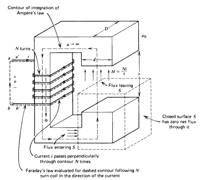
The H field can then only be nonzero in the air gap. This field emanates perpendicularly from the pole faces as no surface currents are present so that the tangential component of H is continuous and thus zero. If we neglect fringing field effects, assuming the gap s to be much smaller than the width d or depth D, the H field is uniform throughout the gap. Using Ampere's circuital law with the contour shown, the only nonzero contribution is in the air gap,
\[\oint_{L} \textbf{H} \cdot \textbf{dl} = Hs = I_{\textrm{total enclosed}} = Ni \]
where we realize that the coil current crosses perpendicularly through our contour N times. The total flux in the air gap is then
\[\Phi = \mu_{0} HDd= \frac{\mu_{0} NDd}{s}i \]
Because the total flux through any closed surface is zero,
\[\oint_{S} \textbf{B} \cdot \textbf{dS} = 0 \]
all the flux leaving S in Figure 6-8 on the air gap side enters the surface through the iron core, as we neglect leakage flux in the fringing field. The flux at any cross section in the iron core is thus constant, given by (3).
If the coil current \(i\) varies with time, the flux in (3) also varies with time so that a voltage is induced across the coil. We use the integral form of Faraday's law for a contour that lies within the winding with Ohmic conductivity \(\sigma\), cross sectional area A, and total length \(l\). Then the current density and electric field within the wire is
\[J = \frac{i}{A}, \: \: \: \: E = \frac{J}{\sigma} = \frac{i}{\sigma A} \]
so that the electromotive force has an Ohmic part as well as a contribution due to the voltage-across the terminals:
\[\oint_{L} \textbf{E} \cdot \textbf{dl} = \int_{a'}^{b'} \underbrace{\frac{i}{\sigma A} dl}_{iR\\ \textrm{in wire}} + \int_{b}^{a} \underbrace{\textbf{E} \cdot \textbf{dl}}_{-v \\ \textrm{across terminals}} = - \frac{d}{dt} \int_{S} \textbf{B} \cdot \textbf{dS} \]
The surface S on the right-hand side is quite complicated because of the spiral nature of the contour. If the coil only had one turn, the right-hand side of (6) would just be the time derivative of the flux of (3). For two turns, as in Figure 6-9, the flux links the coil twice, while for N turns the total flux
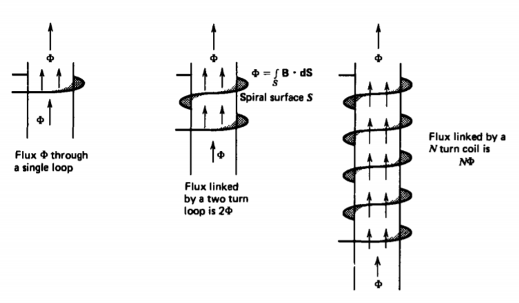
linked by the coil is \(N \Phi\). Then (6) reduces to
\[v = iR + L \frac{di}{dt} \]
where the self-inductance is defined as
\[L = \frac{N \Phi}{i} = \frac{N \int_{S} \textbf{B} \cdot \textbf{dS}}{\oint_{L} \textbf{H} \cdot \textbf{dl}} = \frac{\mu_{0} N^{2} Dd}{s} \textrm{henry} [\textrm{kg m}^{2} \textrm{ A}^{-2} \textrm{ s}^{-2}] \]
For linearly permeable materials, the inductance is always independent of the excitations and only depends on the geometry. Because of the fixed geometry, the inductance is a constant and thus was taken outside the time derivative in (7). In geometries that change with time, the inductance will also be a function of time and must remain under the derivative. The inductance is always proportional to the square of the number of coil turns. This is because the flux \(\Phi\), in the air gap is itself proportional to N and it links the coil N times.
Find the self-inductances for the coils shown in Figure 6-10.
(a) Solenoid
An N turn coil is tightly wound upon a cylindrical core of radius a, length l, and permeability \(\mu\).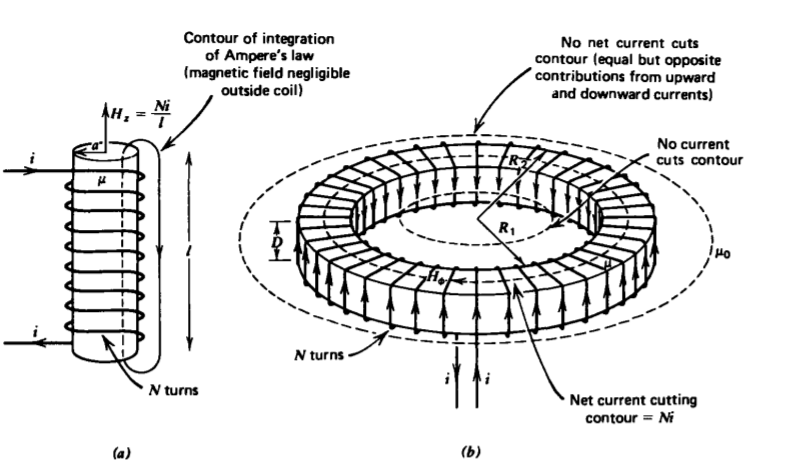
Figure 6-10 Inductances. (a) Solenoidal coil; (b) toroidal coil.
(b) Toroid
An N turn coil is tightly wound around a donut-shaped core of permeability \(\mu\) with a rectangular cross section and inner and outer radii R1 and R2.
Solution
a)
A current i flowing in the wire approximates a surface current
\[K_{\phi} = Ni/l \nonumber \]
If the length l is much larger than the radius a, we can neglect fringing field effects at the ends and the internal magnetic field is approximately uniform and equal to the surface current,
\[H_{z} = K_{\phi} = \frac{Ni}{l} \nonumber \]
as we assume the exterior magnetic field is negligible. The same result is obtained using Ampere's circuital law for the contour shown in Figure 6-10a. The flux links the coil N times:
\[L = \frac{N \Phi}{i} = \frac{N \mu H_{z} \pi a^{2}}{i} = \frac{N^{2} \mu \pi a^{2}{l} \nonumber \]
b) Applying Ampere's circuital law to the three contours shown in Figure 6-10b, only the contour within the core has a net current passing through it:
\[\oint_{L} \textbf{H} \cdot \textbf{dl} = H_{\phi} 2 \pi \textrm{r} = \left \{ \begin{matrix} 0, & \textrm{r} < R_{1} \\ Ni, & R_{1} < \textrm{r} < R_{2} \\ 0, & \textrm{r} > R_{2} \end{matrix} \right. \nonumber \]
The inner contour has no current through it while the outer contour enclosing the whole toroid has equal but opposite contributions from upward and downward currents.
The flux through any single loop is
\[\Phi = \mu D \int_{R_{1}}^{R_{2}} H_{\phi} d \textrm{r} \\ = \frac{\mu D N i }{2 \pi} \int_{R_{1}}^{R_{2}} \frac{d \textrm{r}}{\textrm{r}} \\ = \frac{\mu D Ni}{2 \pi} \ln \frac{R_{2}}{R_{1}} \nonumber \]
so that the self-inductance is
\[L = \frac{N \Phi}{i} = \frac{\mu D N^{2}}{2 \pi} \ln \frac{R_{2}}{R_{1}} \nonumber \]
6-2-2 Reluctance
Magnetic circuits are analogous to resistive electronic circuits if we define the magnetomotive force (MMF) \(\mathcal{F}\) analogous to the voltage (EMF) as
\[\mathscr{F} = Ni \]
The flux then plays the same role as the current in electronic circuits so that we define the magnetic analog to resistance as the reluctance:
\[\mathscr{R} = \frac{\mathscr{F}}{\Phi} = \frac{N^{2}}{L} = \frac{(\textrm{length})}{(\textrm{permeatbility})(\textrm{cross-sectional area})} \]
which is proportional to the reciprocal of the inductance.
The advantage to this analogy is that the rules of adding reluctances in series and parallel obey the same rules as resistances.
(a) Reluctances in Series
For the iron core of infinite permeability in Figure 6-11 a, with two finitely permeable gaps the reluctance of each gap is found from (8) and (10) as
\[\mathscr{R}_1=\frac{s_1}{\mu_1 a_1 D}, \quad \mathscr{R}_2=\frac{s_2}{\mu_2 a_2 D}\]
so that the flux is
\[\Phi = \frac{\mathscr{F}}{\mathscr{R}_{1} + \mathscr{R}_{2}} = \frac{Ni}{\mathscr{1} + \mathscr{2}} \Rightarrow L = \frac{N \Phi}{i} = \frac{N^{2}}{\mathscr{R}_{1} + \mathscr{R}_{2}} \]
The iron core with infinite permeability has zero reluctance. If the permeable gaps were also iron with infinite permeability, the reluctances of (11) would also be zero so that the flux
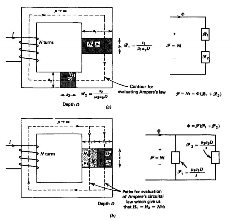
in (12) becomes infinite. This is analogous to applying a voltage across a short circuit resulting in an infinite current. Then the small resistance in the wires determines the large but finite current. Similarly, in magnetic circuits the small reluctance of a closed iron core of high permeability with no gaps limits the large but finite flux determined by the saturation value of magnetization.
The H field is nonzero only in the permeable gaps so that Ampere's law yields
\[H_{1}s_{1} + H_{2}s_{2} = Ni \]
Since the flux must be continuous at every cross section,
\[\Phi = \mu_{1} H_{1} a_{1}D = \mu_{2} H_{2} a_{2}D \]
we solve for the H fields as
\[H_{1} = \frac{\mu_{2} a_{2} Ni}{\mu_{1}a_{1}s_{2} + \mu_{2}a_{2}s_{1}}, \: \: \: \: H_{2} \frac{mu_{1}a_{1}Ni}{\mu_{1}a_{1}s_{2} + \mu_{2}a_{2}s_{1}} \]
(b) Reluctances in Parallel
If a gap in the iron core is filled with two permeable materials, as in Figure 6-1 lb, the reluctance of each material is still given by (11). Since each material sees the same magnetomotive force, as shown by applying Ampere's circuital law to contours passing through each material,
\[H_{1}s = H_{2}s = N_{i} \Rightarrow H_{1} = H_{2} = \frac{Ni}{s} \]
the H fields in each material are equal. The flux is then
\[\Phi = (\mu_{1} H_{1} a_{1} + \mu_{2} H_{2} a_{2}) D = \frac{Ni(\mathscr{R}_{1} + \mathscr{R}_{2})}{\mathscr{R}_{1} \mathscr{R}_{2}} = Ni (\mathscr{P}_{1} + \mathscr{P}_{2}) \]
where the permeances \(\mathscr{P}_{1}\) and \(\mathscr{P}_{2}\) are just the reciprocal reluctances analogous to conductance.
6-2-3 Transformer Action
(a) Voltages are not Unique
Consider two small resistors \(R_{1}\) and \(R_{2}\) forming a loop enclosing one leg of a closed magnetic circuit with permeability \(\mu\), as in Figure 6-12. An N turn coil excited on one leg with a time varying current generates a time varying flux that is approximately
\[\Phi(t) = \mu N A i_{1}/l \]
where \(l\) is the average length around the core.
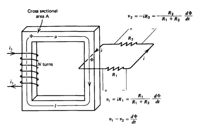
Applying Faraday's law to the resistive loop we have
\[\oint_{L} \textbf{E} \cdot \textbf{dl} = i (R_{1} + R_{2}) = + \frac{d \Phi (t)}{dt} \Rightarrow i = \frac{1}{R_{1} + R_{2}} \frac{d \Phi}{dt} \]
where we neglect the self-flux produced by the induced current \(i\) and reverse the sign on the magnetic flux term because \(\Phi\) penetrates the loop in Figure 6-12 in the direction opposite to the positive convention given by the right-hand rule illustrated in Figure 6-2.
If we now measured the voltage across each resistor, we would find different values and opposite polarities even though our voltmeter was connected to the same nodes:
\[v_{1} = iR_{1} = + \frac{R_{1}}{R_{1} + R_{2}} \frac{d \Phi}{dt} \\ v_{2} = - R_{2} = \frac{-R_{2}}{R_{1}+ R_{2}} \frac{d \Phi}{dt} \]
This nonuniqueness of the voltage arises because the electric field is no longer curl free. The voltage difference between two points depends on the path of the connecting wires. If any time varying magnetic flux passes through the contour defined by the measurement, an additional contribution results.
(b) Ideal Transformers
Two coils tightly wound on a highly permeable core, so that all the flux of one coil links the other, forms an ideal transformer, as in Figure 6-13. Because the iron core has an infinite permeability, all the flux is confined within the core. The currents flowing in each coil, \(i_{1}\) and \(i_{2}\), are defined so that when they are positive the fluxes generated by each coil are in the opposite direction. The total flux in the core is then
\[\Phi = \frac{N_{1}i_{1} - N_{2}i_{2}}{\mathscr{R}}, \: \: \: \: \mathscr{R} = \frac{l}{\mu A} \]
where \(\mathscr{R}\) is the reluctance of the core and \(l\) is the average length of the core.
The flux linked by each coil is then
\[\lamba_{1} = N_{1} \Phi = \frac{\mu A}{l} (N_{1}^{2} i_{1} - N_{1} N_{2} i_{2}) \\ \lambda_{2} = N_{2} \Phi = \frac{\mu A}{l} (N_{1}N_{2}i_{1} - N_{2}^{2} i_{2}) \]
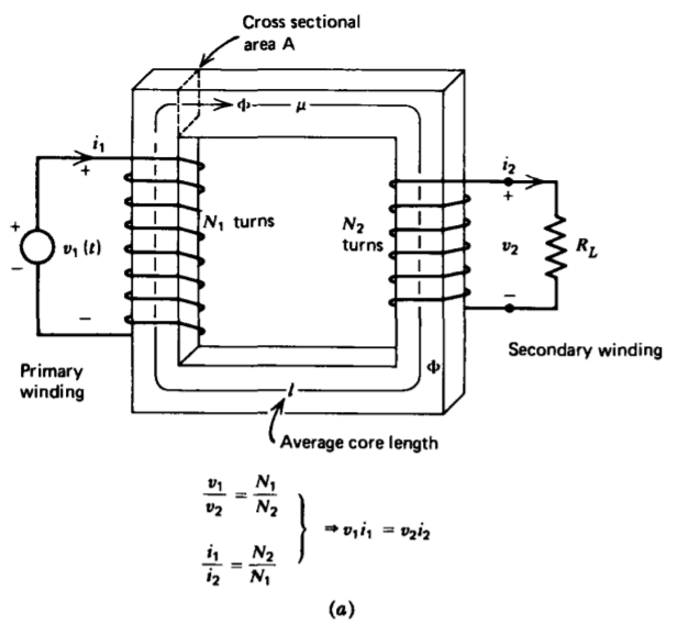
which can be written as
\[\lambda_{1} = L_{1}i_{1}- M i_{2} \\ \lambda_{2} = M i_{1} - L_{2} i_{2} \]
where \(L_{1}\) and \(L_{2}\) are the self-inductances of each coil alone and M is the mutual inductance between coils:
\[L_{1} = N_{1}^{2} L_{0}, \: \: \: \: L_{2} = N_{2}^{2}L_{0}, \: \: \: \: M = N_{1} N_{2}L_{0}, \: \: \: \: L_{0} = \mu A/l \]
In general, the mutual inductance obeys the equality:
\[M = k(L_{1}L_{2})^{1/2}, \: \: \: \: 0 \leq k \leq 1 \]
where k is called the coefficient of coupling. For a noninfinite core permeability, k is less than unity because some of the flux of each coil goes into the free space region and does not link the other coil. In an ideal transformer, where the permeability is infinite, there is no leakage flux so that k = 1.
From (23), the voltage across each coil is
\[v_{1} = \frac{d \lambda_{1}}{dt} = L_{1} \frac{di_{1}}{dt} - M \frac{di_{2}}{dt} \\ v_{2} = \frac{d \lambda_{2}}{dt} = M \frac{di_{1}}{dt} - L_{2} \frac{di_{2}}{dt} \]
Because with no leakage, the mutual inductance is related to the self-inductances as
\[M = \frac{N_{2}}{N_{1}} L_{1} = \frac{N_{1}}{N_{2}} L_{2} \]
the ratio of coil voltages is the same as the turns ratio:
\[\frac{v_{1}}{v_{2}} = \frac{d \lambda_{1}/dt}{d \lambda_{2}/dt} = \frac{N_{1}}{N_{2}} \]
In the ideal transformer of infinite core permeability, the inductances of (24) are also infinite. To keep the voltages and fluxes in (26) finite, the currents must be in the inverse turns ratio
\[\frac{i_{1}}{i_{2}} = \frac{N_{2}}{N_{1}} \]
The electrical power delivered by the source to coil 1, called the primary winding, just equals the power delivered to the load across coil 2, called the secondary winding:
\[v_{1} i_{1} = v_{2}i_{2} \]
If \(N_{2} > N_{1}\), the voltage on winding 2 is greater than the voltage on winding 1 but current \(i_{2}\) is less than \(i_{1}\) keeping the powers equal.
If primary winding 1 is excited by a time varying voltage \(v_{1}(t)\) with secondary winding 2 loaded by a resistor \(R_{L}\) so that
\[v_{2} = i_{2}R_{L} \]
the effective resistance seen by the primary winding is
\[R_{\textrm{eff}} = \frac{v_{1}}{i_{1}} = \frac{N_{1}}{N_{2}} \frac{v_{2}}{(N_{2}/N_{1})i_{2}} = \bigg(\frac{N_{1}}{N_{2}} \bigg)^{2} R_{L} \]
A transformer is used in this way as an impedance transformer where the effective resistance seen at the primary winding is increased by the square of the turns ratio.
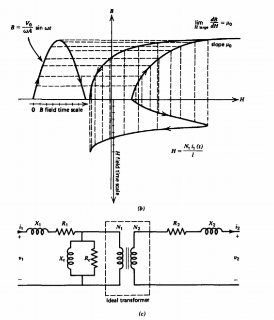
(c) Real Transformers
When the secondary is open circuited (i2= 0), (29) shows that the primary current of an ideal transformer is also zero. In practice, applying a primary sinusoidal voltage \(V_{0} \cos \omega t\) will result in a small current due to the finite self-inductance of the primary coil. Even though this self-inductance is large if the core permeability \(\mu\) is large, we must consider its effect because there is no opposing flux as a result of the open circuited secondary coil. Furthermore, the nonlinear hysteresis curve of the iron as discussed in Section 5-5-3c will result in a nonsinusoidal current even though the voltage is sinusoidal. In the magnetic circuit of Figure 6.13a with \(i_{2} = 0\), the magnetic field is
\[\textbf{H} = \frac{N_{1}i_{1}}{l} \]
while the imposed sinusoidal voltage also fixes the magnetic flux to be sinusoidal
\[v_{1} = \frac{d \Phi}{dt} = V_{0} \cos \omega t \Rightarrow \Phi = BA = \frac{V_{0}}{\omega} \sin \omega t \]
Thus the upper half of the nonlinear B-H magnetization characteristic in Figure 6-13b has the same shape as the flux-current characteristic with proportionality factors related to the geometry. Note that in saturation the B-H curve approaches a straight line with slope \(\mu_{0}\). For a half-cycle of flux given by (34), the nonlinear open circuit magnetizing current is found graphically as a function of time in Figure 6-13b. The current is symmetric over the negative half of the flux cycle. Fourier analysis shows that this nonlinear current is composed of all the odd harmonics of the driving frequency dominated by the third and fifth harmonics. This causes problems in power systems and requires extra transformer windings to trap the higher harmonic currents, thus preventing their transmission.
A more realistic transformer equivalent circuit is shown in Figure 6-13c where the leakage reactances \(X_{1}\) and \(X_{2}\) represent the fact that all the flux produced by one coil does not link the other. Some small amount of flux is in the free space region surrounding the windings. The nonlinear inductive reactance \(X_{c}\) represents the nonlinear magnetization characteristic illustrated in Figure 6-13b, while \(R_{c}\) represents the power dissipated in traversing the hysteresis loop over a cycle. This dissipated power per cycle equals the area enclosed by the hysteresis loop. The winding resistances are \(R_{1}\) and \(R_{2}\).