6.3: Energy Stored in the Magnetic Field

6-3-1 The Electric Field Transformation

If a point charge q travels with a velocity v through a region with electric field E and magnetic field B, it experiences the combined Coulomb-Lorentz force

\[\textbf{F} = q (\textbf{E} + \textbf{v} \times \textbf{B}) \]

Now consider another observer who is travelling at the same velocity v as the charge carrier so that their relative velocity is zero. This moving observer will then say that there is no Lorentz force, only a Coulombic force

\[\textbf{F}' = q \textbf{E}' \]

where we indicate quantities measured by the moving observer with a prime. A fundamental postulate of mechanics is that all physical laws are the same in every inertial coordinate system (systems that travel at constant relative velocity). This requires that the force measured by two inertial observers be the same so that F'= F:

\[\textbf{E}' = \textbf{E} + \textbf{v} \times \textbf{B} \]

The electric field measured by the two observers in relative motion will be different. This result is correct for material velocities much less than the speed of light and is called a Galilean field transformation. The complete relativistically correct transformation slightly modifies (3) and is called a Lorentzian transformation but will not be considered here.

In using Faraday's law of Section 6-1-1, the question remains as to which electric field should be used if the contour L and surface S are moving. One uses the electric field that is measured by an observer moving at the same velocity as the convecting contour. The time derivative of the flux term cannot be brought inside the integral if the surface S is itself a function of time.

6-3-2 Ohm's Law for Moving Conductors

The electric field transformation of (3) is especially important in modifying Ohm's law for moving conductors. For nonrelativistic velocities, an observer moving along at the same velocity as an Ohmic conductor measures the usual Ohm's law in his reference frame,

\[\textbf{J}_{f}' = \sigma \textbf{E}' \]

where we assume the conduction process is unaffected by the motion. Then in Galilean relativity for systems with no free charge, the current density in all inertial frames is the same so that (3) in (4) gives us the generalized Ohm's law as

\[\textbf{J}_{f}' = \textbf{J}_{f} = \sigma (\textbf{E} + \textbf{v} \times \textbf{B}) \]

where v is the velocity of the conductor.

The effects of material motion are illustrated by the parallel plate geometry shown in Figure 6-14. A current source is applied at the left-hand side that distributes itself uniformly as a surface current \(K_{x} = \pm I/D\) on the planes. The electrodes are connected by a conducting slab that moves to the right with constant velocity U. The voltage across the current source can be computed using Faraday's law with the contour shown. Let us have the contour continually expanding with the 2-3 leg moving with the conductor. Applying Faraday's law we have

\[\oint_{L} \textbf{E}' \cdot \textbf{dl} = \int_{1}^{2} \textbf{E} \nearrow^{0} \cdot \textbf{dl} + \int_{2}^{3} \underbrace{\textbf{E}' \cdot \textbf{dl}}_{iR} + \int_{3}^{4} \textbf{e} \nearrow^{0} \cdot \textbf{dl} + \int_{4}^{1} \underbrace{\textbf{E} \cdot \textbf{dl}}_{- \nu} \\ = - \frac{d}{dt} \int_{S} \textbf{B} \cdot \textbf{dS} \]

Figure 6-14 A moving, current-carrying Ohmic conductor generates a speed voltage as well as the usual resistive voltage drop.

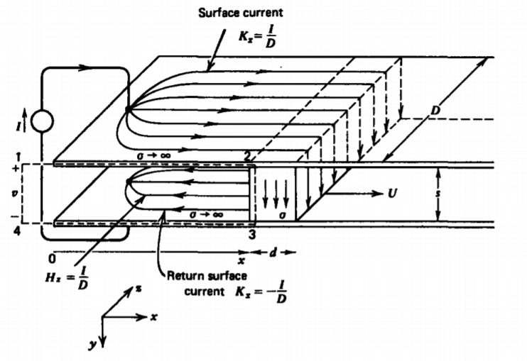
where the electric field used along each leg is that measured by an observer in the frame of reference of the contour. Along the 1-2 and 3-4 legs, the electric field is zero within the stationary perfect conductors. The second integral within the moving Ohmic conductor uses the electric field E', as measured by a moving observer because the contour is also expanding at the same velocity, and from (4) and (5) is related to the terminal current as

\[\textbf{E}' = \frac{\textbf{J}'}{\sigma} = \frac{I}{\sigma Dd} \textbf{i}_{y} \]

In (6), the last line integral across the terminals defines the voltage.

\[\frac{Is}{\sigma Dd} - v = - \frac{d}{dt} \int_{S} \textbf{B} \cdot \textbf{dS} = - \frac{d}{dt} (\mu_{0} H_{z} xs) \]

The first term is just the resistive voltage drop across the conductor, present even if there is no motion. The term on the right-hand side in (8) only has a contribution due to the linearly increasing area (\(dx/dt = U\)) in the free space region with constant magnetic field,

\[H_{z} = I/D \]

The terminal voltage is then

\[ v = I \bigg( R + \frac{\mu_{0}Us}{D} \bigg) , \: \: \: R = \frac{s}{\sigma Dd} \]

We see that the speed voltage contribution arose from the flux term in Faraday's law. We can obtain the same solution using a contour that is stationary and does not expand with the conductor. We pick the contour to just lie within the conductor at the time of interest. Because the contour does not expand with time so that both the magnetic field and the contour area does not change with time, the right-hand side of (6) is zero. The only difference now is that along the 2-3 leg we use the electric field as measured by a stationary observer,

\[\textbf{E} = \textbf{E}' - \textbf{v} \times \textbf{B} \]

so that (6) becomes

\[IR + \frac{\mu_{0} UIs}{D} - v = 0 \]

which agrees with (10) but with the speed voltage term now arising from the electric field side of Faraday's law.

This speed voltage contribution is the principle of electric generators converting mechanical work to electric power when moving a current-carrying conductor through a magnetic field. The resistance term accounts for the electric power dissipated. Note in (10) that the speed voltage contribution just adds with the conductor's resistance so that the effective terminal resistance is \(v/I = R + (\mu_{o} Us/D)\). If the slab moves in the opposite direction such that U is negative, the terminal resistance can also become negative for sufficiently large \(U \: (U < -RD/\mu_{0}s)\). Such systems are unstable where the natural modes grow rather than decay with time with any small perturbation, as illustrated in Section 6-3-3b.

6-3-3 Faraday's Disk (Homopolar Generator)*

(a) Imposed Magnetic Field

A disk of conductivity \(\sigma\) rotating at angular velocity \(\omega\) transverse to a uniform magnetic field \(B_{0} \textbf{i}_{z}\), illustrates the basic principles of electromechanical energy conversion. In Figure 6-15a we assume that the magnetic field is generated by an N turn coil wound on the surrounding magnetic circuit,

\[B_{0} = \frac{\mu_{0} Ni_{f}}{s} \]

The disk and shaft have a permeability of free space \(\mu_{0}\), so that the applied field is not disturbed by the assembly. The shaft and outside surface at r = \(R_{0}\) are highly conducting and make electrical connection to the terminals via sliding contacts.

We evaluate Faraday's law using the contour shown in Figure 6-15a where the 1-2 leg within the disk is stationary so the appropriate electric field to be used is given by (11):

\[E_{\textrm{r}} = \frac{J_{\textrm{r}}}{\sigma} - \omega \textrm{r} B_{0} = \frac{i_{r}}{2 \pi \sigma d \textrm{r}} - \omega \textrm{r} B_{0} \]

where the electric field and current density are radial and i, is the total rotor terminal current. For the stationary contour with a constant magnetic field, there is no time varying flux through the contour:

\[\oint_{L} \textbf{E} \cdot \textbf{dl} = \int_{1}^{2} E_{\textrm{r}} d \textrm{r} + \int_{3}^{4} \underbrace{\textbf{E} \cdot \textbf{dl}}_{-v_{r}} = 0 \]

Figure 6-15 (a) A conducting disk rotating in an axial magnetic field is called a homopolar generator. (b) In addition to Ohmic and inductive voltages there is a speed voltage contribution proportional to the speed of the disk and the magnetic field.

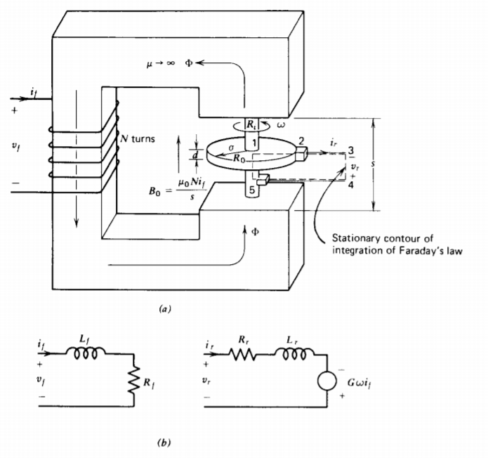
Using (14) in (15) yields the terminal voltage as

\[v_{r} = \int_{R_{i}}^{R_{0}} \bigg( \frac{i_{r}}{2 \pi \textrm{r} \sigma d} - \omega \textrm{r} B_{0} \bigg) d \textrm{r} \\ \frac{i_{r}}{2 \pi \sigma d} \ln \frac{R_{0}}{R_{i}} - \frac{\omega B_{0}}{2} (R_{0}^{2}-R_{i}^{2}) \\ = i_{r}R_{r} - G \omega i_{f} \]

where \(R_{r}\) is the internal rotor resistance of the disk and G is called the speed coefficient:

\[R_{r} = \frac{\ln (R_{0}/R_{i})}{2 \pi \sigma d}, \: \: \: G = \frac{\mu_{0}N}{2s} (R_{0}^{2} - R_{i}^{2}) \]

We neglected the self-magnetic field due to the rotor current, assuming it to be much smaller than the applied field \(B_{0}\), but it is represented in the equivalent rotor circuit in Figure 6-15b as the self-inductance \(L_{r}\) in series with a resistor and a speed voltage source linearly dependent on the field current. The stationary field coil is represented by its self-inductance and resistance.

For a copper disk (\(\sigma \approx 6 \times 10^{7}\) siemen/m) of thickness 1mm rotating at 3600 rpm (\(\omega \approx 120 \pi\) radian/sec) with outer and inner radii \(R_{0} = 10\)cm and \(R_{i} = 1\)cm in a magnetic field of \(B_{0}\) = 1 tesla, the open circuit voltage is

\[v_{\alpha} = - \frac{\omega B_{0}}{2}(R_{0}^{2} - R_{i}^{2}) \approx -1.9 \textrm{V} \]

while the short circuit current is

\[i_{\textrm{sc}} = \frac{v_{\textrm{oc}}}{\ln (R_{0}/R_{i})} 2 \pi \sigma d \approx 3 \times 10^{5} \textrm{amp} \]

Homopolar generators are typically high current, low voltage devices. The electromagnetic torque on the disk due to the Lorentz force is

\[\textbf{T} = \int_{\phi = 0}^{2 \pi} \int_{z=0}^{d} \int_{\textrm{r} = R_{i}}^{R_{0}} \textrm{r} \textbf{i}_{\textrm{r}} \times (\textbf{J} \times \textbf{B}) \textrm{r} d \textrm{r} d \phi d z \\ = -r_{r}B_{0} \textbf{i}_{z} \int_{R_{i}}^{R_{0}} \textrm{r} d \textrm{r} \\ = - \frac{i_{r} B_{0}}{2} (R_{0}^{2} - R_{i}^{2}) \textbf{i}_{z} \\ = - G i_{f} i_{r} \textbf{i}_{z} \]

The negative sign indicates that the Lorentz force acts on the disk in the direction opposite to the motion. An external torque equal in magnitude but opposite in direction to (20) is necessary to turn the shaft.

This device can also be operated as a motor if a rotor current into the disk (\(i_{r} < 0\)) is imposed. Then the electrical torque causes the disk to turn.

(b) Self-Excited Generator

For generator operation it is necessary to turn the shaft and supply a field current to generate the magnetic field. However, if the field coil is connected to the rotor terminals, as in Figure 6-16a, the generator can supply its own field current. The equivalent circuit for self-excited operation is shown in Figure 6-16b where the series connection has \(i_{r} = i_{f}\).

Figure 6-16 A homopolar generator can be self-excited where the generated rotor current is fed back to the field winding to generate its own magnetic field.

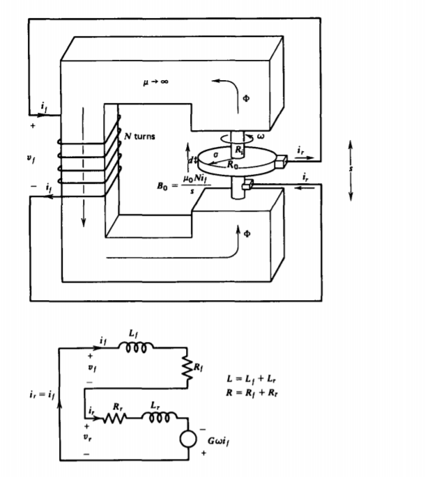
Kirchoff's voltage law around the loop is

\[L \frac{di}{dt} + i(R-G \omega) = 0, \: \: \: \: R = R_{r} + R_{f}, \: \: \: \: L = L_{r} + L_{f} \]

where R and L are the series resistance and inductance of the coil and disk. The solution to (21) is

\[ i=I_0 e^{-[(R-G \omega) / L] t} \]

where \(I_{0}\) is the initial current at t = 0. If the exponential factor is positive

\[G \omega > R \]

the current grows with time no matter how small \(I_{0}\) is. In practice, \(I_{0}\) is generated by random fluctuations (noise) due to residual magnetism in the iron core. The exponential growth is limited by magnetic core saturation so that the current reaches a steady-state value. If the disk is rotating in the opposite direction (\(\omega\) <0), the condition of (23) cannot be satisfied. It is then necessary for the field coil connection to be reversed so that \(i_{r} = -i_{f}\). Such a dynamo model has been used as a model of the origin of the earth's magnetic field.

(c) Self-Excited ac Operation

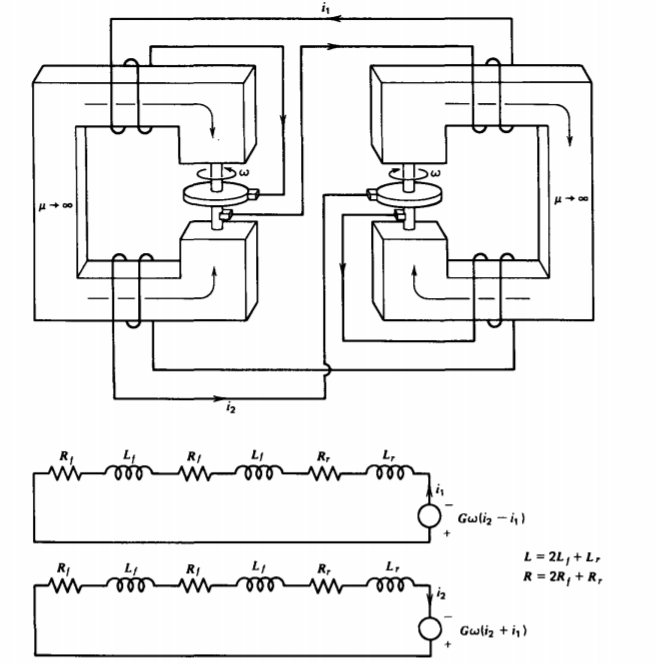
Two such coupled generators can spontaneously generate two phase ac power if two independent field windings are connected, as in Figure 6-17. The field windings are connected so that if the flux through the two windings on one machine add, they subtract on the other machine. This accounts for the sign difference in the speed voltages in the equivalent circuits,

\[L = \frac{di_{1}}{dt} + (R-G \omega) i_{1} + G \omega i_{2} = 0 \\ L \frac{di_{2}}{dt} + (R-G \omega) i_{2} - G \omega i_{1} = 0 \]

where L and R are the total series inductance and resistance. The disks are each turned at the same angular speed \(\omega\).

Since (24) are linear with constant coefficients, solutions are of the form

\[i_{1} = I_{1} e^{st}, \: \: \: \: i_{2} = I_{2} e^{st} \]

which when substituted back into (24) yields

\[(Ls + R - G \omega) I_{1} + G \omega I_{2} = 0 \\ -G \omega I_{1} + (Ls + R - G \omega) I_{2} = 0 \]

For nontrivial solutions, the determinant of the coefficients of \(I_{1}\) and \(I_{2}\) must be zero,

\[(Ls + R - G \omega)^{2} = -(G \omega)^{2} \]

which when solved for s yields the complex conjugate natural frequencies,

\[s = - \frac{(R- G \omega)}{L} \pm j \frac{G \omega}{L} \\ I_{1}/I_{2} = \pm j \]

where the currents are 90° out of phase. If the real part of s is positive, the system is self-excited so that any perturbation

Figure 6-17 Cross-connecting two homopolar generators can result in self-excited two-phase alternating currents. Two independent field windings are required where on one machine the fluxes add while on the other they subtract.

grows at an exponential rate:

\[G \omega > R \]

The imaginary part of s yields the oscillation frequency

\[\omega_{0} = \textrm{Im} (s) = G \omega/L \]

Again, core saturation limits the exponential growth so that two-phase power results. Such a model may help explain the periodic reversals in the earth's magnetic field every few hundred thousand years.

(d) Periodic Motor Speed Reversals

If the field winding of a motor is excited by a dc current, as in Figure 6-18, with the rotor terminals connected to a generator whose field and rotor terminals are in series, the circuit equation is

\[\frac{di}{dt} + \frac{(R - G_{g}\omega_{g})}{L} i = \frac{G_{m} \omega_{m}}{L} I_{f} \]

where L and R are the total series inductances and resistances. The angular speed of the generator \(\omega_{g}\) is externally

Figure 6-18 Cross connecting a homopolar generator and motor can result in spontaneous periodic speed reversals of the motor's shaft.

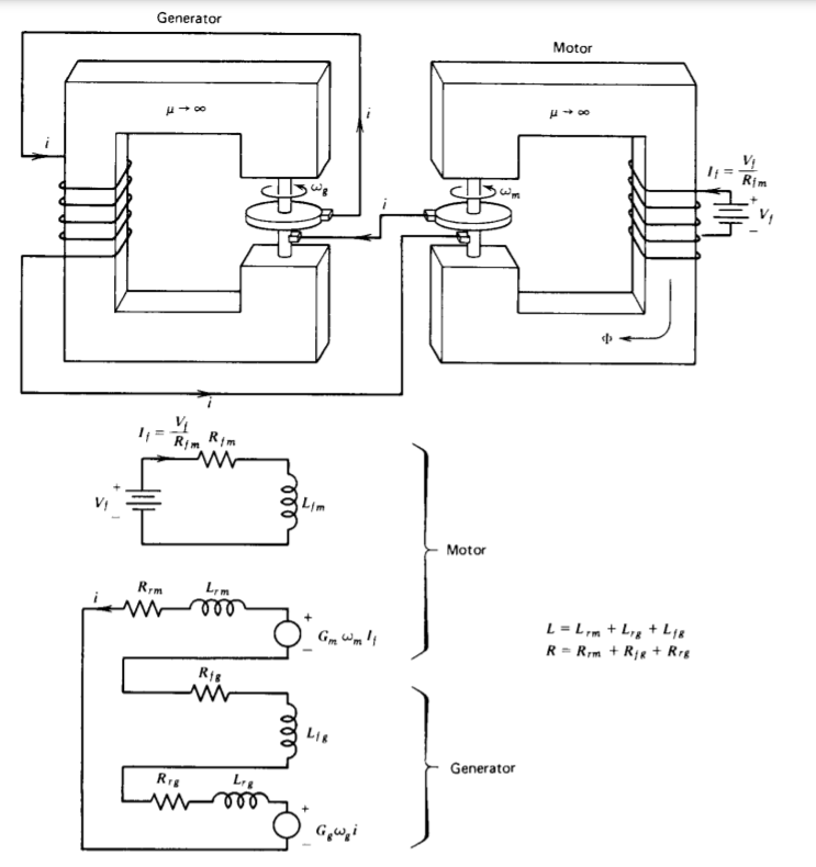
constrained to be a constant. The angular acceleration of the motor's shaft is equal to the torque of (20),

\[J \frac{d \omega_{m}}{dt} = - G_{m}I_{f}i \]

where J is the moment of inertia of the shaft and \(I_{f} = V_{f}/R_{fm}\) is the constant motor field current.

Solutions of these coupled, linear constant coefficient differential equations are of the form

\[i = I e^{st} \\ \omega = W e^{st} \]

which when substituted back into (31) and (32) yield

\[I \bigg( s + \frac{R - G_{g} \omega_{g}}{L} \bigg) - W \bigg(\frac{G_{m}I_{f}}{L} \bigg) = 0 \\ I \bigg( \frac{G_{m} I_{f}}{J} \bigg) + W s = 0 \]

Again, for nontrivial solutions the determinant of coefficients of I and W must be zero,

\[s \bigg(s + \frac{R - G_{g} \omega_{g}}{L} \bigg) + \frac{(G_{m} I_{f})^{2}}{JL} =0 \]

which when solved for s yields

\[s = - \frac{(R - G_{g} \omega_{g})}{2L} \pm \bigg[ \bigg( \frac{R-G_{g}\omega_{g}}{2L} \bigg)^{2} - \frac{(G_{m}I_{f})^{2}}{JL} \bigg]^{1/2} \]

For self-excitation the real part of s must be positive,

\[G_{g} \omega_{g} > R \]

while oscillations will occur if s has an imaginary part,

\[\frac{(G_{m}I_{f})^{2}}{JL} > \bigg( \frac{R-G_{g}\omega_{g}}{2L} \bigg)^{2} \]

Now, both the current and shaft's angular velocity spontaneously oscillate with time.

* Some of the treatment in this section is similar to that developed in: H. H. Woodson and J. R. Melcher, Electromechanical Dynamics, Part I, Wiley, N. Y., 1968, Ch. 6

6-3-4 Basic Motors and Generators

(a) ac Machines

Alternating voltages are generated from a dc magnetic field by rotating a coil, as in Figure 6-19. An output voltage is measured via slip rings through carbon brushes. If the loop of area A is vertical at t = 0 linking zero flux, the imposed flux

Figure 6-19 A coil rotated within a constant magnetic field generates a sinusoidal voltage.

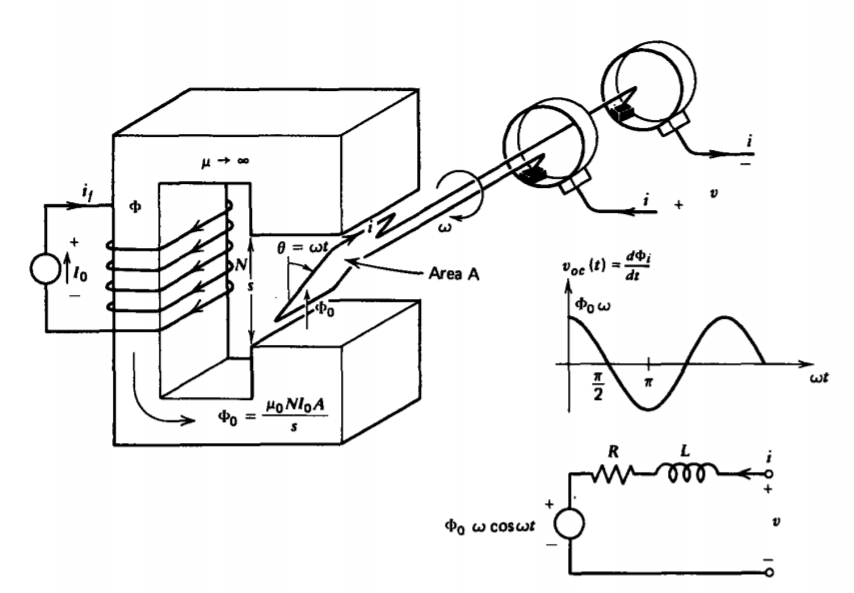
through the loop at any time, varies sinusoidally with time due to the rotation as

\[\Phi_{i} = \Phi_{0} \sin \omega t \]

Faraday's law applied to a stationary contour instantaneously passing through the wire then gives the terminal voltage as

\[v = iR + \frac{d \Phi}{dt} = iR + L \frac{di}{dt} + \Phi_{0} \omega \cos \omega t \]

where R and L are the resistance and inductance of the wire. The total flux is equal to the imposed flux of (39) as well as self-flux (accounted for by L) generated by the current i. The equivalent circuit is then similar to that of the homopolar generator, but the speed voltage term is now sinusoidal in time

(b) dc Machines

DC machines have a similar configuration except that the slip ring is split into two sections, as in Figure 6-20a. Then whenever the output voltage tends to change sign, the terminals are also reversed yielding the waveform shown, which is of one polarity with periodic variations from zero to a peak value.

Figure 6-20 (a) If the slip rings are split so that when the voltage tends to change sign the terminals are also reversed, the resulting voltage is of one polarity. (b) The voltage waveform can be smoothed out by placing a second coil at right angles to the first and using a four-section commutator.

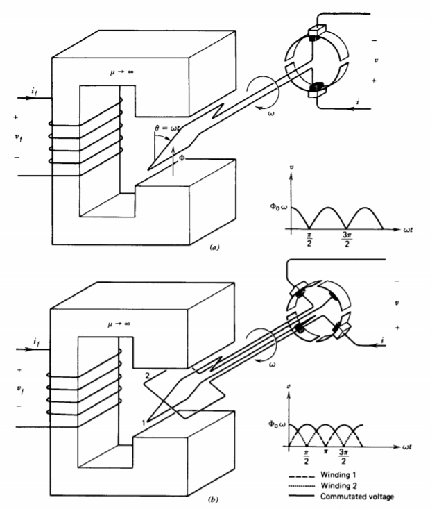
The voltage waveform can be smoothed out by using a four-section commutator and placing a second coil perpendicular to the first, as in Figure 6-20b. This second coil now generates its peak voltage when the first coil generates zero voltage. With more commutator sections and more coils, the dc voltage can be made as smooth as desired.

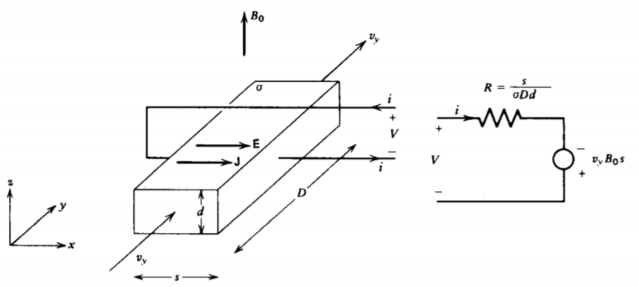
6-3-5 MHD Machines

Magnetohydrodynamic machines are based on the same principles as rotating machines, replacing the rigid rotor by a conducting fluid. For the linear machine in Figure 6-21, a fluid with Ohmic conductivity \(\sigma\) flowing with velocity \(v_{y}\) moves perpendicularly to an applied magnetic field \(B_{0} \textbf{i}_{z}\). The terminal voltage V is related to the electric field and current as

\[\textbf{E} = \textbf{i}_{x} \frac{V}{s}, \: \: \: \: \textbf{J} = \sigma (\textbf{E} + \textbf{v} \times \textbf{B}) = \sigma \bigg( \frac{V}{s} + v_{y}B_{0} \bigg) \textbf{i}_{x} = \frac{i}{Dd} \textbf{i}_{x} \]

which can be rewritten as

\[V = iR - v_{y} B_{0}s \]

which has a similar equivalent circuit as for the homopolar generator.

The force on the channel is then

\[\textbf{f} = \int_{\textrm{V}} \textbf{J} \times \textbf{B} d \textrm{V} \\ = -i B_{0} s \textbf{i}_{y} \]

again opposite to the fluid motion.

6-3-6 Paradoxes

Faraday's law is prone to misuse, which has led to numerous paradoxes. The confusion arises because the same

Figure 6-21 An MHD (magnetohydrodynamic) machine replaces a rotating conductor by a moving fluid.

contribution can arise from either the electromotive force side of the law, as a speed voltage when a conductor moves orthogonal to a magnetic field, or as a time rate of change of flux through the contour. This flux term itself has two contributions due to a time varying magnetic field or due to a contour that changes its shape, size, or orientation. With all these potential contributions it is often easy to miss a term or to double count.

(a) A Commutatorless de Machine*

Many persons have tried to make a commutatorless dc machine but to no avail. One novel unsuccessful attempt is illustrated in Figure 6-22, where a highly conducting wire is vibrated within the gap of a magnetic circuit with sinusoidal velocity:

\[v_{x} = v_{0} \sin \omega t \]

Figure 6-22 It is impossible to design a commutatorless dc machine. Although the speed voltage alone can have a dc average, it will be canceled by the transformer electromotive force due to the time rate of change of magnetic flux through the loop. The total terminal voltage will always have a zero time average.

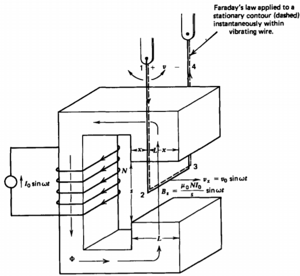
The sinusoidal current imposes the air gap flux density at the same frequency \(\omega\):

\[B_{z} = B_{0} \sin \omega t, \: \: \: \: B_{0} = \mu_{0} NI_{0}/s \]

Applying Faraday's law to a stationary contour instantaneously within the open circuited wire yields

\[ \] \[ \begin{aligned}
\oint_L E \cdot d l & =\int_1^2 E^{\pi^0} \cdot d l+\int_2^3 \underbrace{E \cdot d l}_{E=-v \times B}+\int_3^4 E^{E^0} \cdot d \mathrm{dl}+\int_4^1 \underbrace{E \cdot d l}_{-v} \\
& =-\frac{d}{d t} \int_S B \cdot d S
\end{aligned} \]

where the electric field within the highly conducting wire as measured by an observer moving with the wire is zero. The electric field on the 2-3 leg within the air gap is given by (11), where \(\textbf{E}'=0\) while the 4-1 leg defines the terminal voltage. If we erroneously argue that the flux term on the right-hand side is zero because the magnetic field B is perpendicular to dS, the terminal voltage is

\[v = v_{x} B_{z} l = v_{0} B_{0} l \sin^{2} \omega t \]

which has a dc time-average value. Unfortunately, this result is not complete because we forgot to include the flux that turns the corner in the magnetic core and passes perpendicularly through our contour. Only the flux to the right of the wire passes through our contour, which is the fraction \((L-x)/L\) of the total flux. Then the correct evaluation of (46) is

\[-v + v_{x}B_{z}l = + \frac{d}{dt}[(L-x) B_{z}l] \]

where x is treated as a constant because the contour is stationary. The change in sign on the right-hand side arises because the flux passes through the contour in the direction opposite to its normal defined by the right-hand rule. The voltage is then

\[v = v_{x} B_{z} l - (L-x) l \frac{dB_{z}}{dt} \]

where the wire position is obtained by integrating (44),

\[x = \int v_{x} dt = - \frac{v_{0}}{\omega} (\cos \omega t - 1) + x_{0} \]

and \(x_{0}\) is the wire's position at t = 0. Then (49) becomes

\[v = l \frac{d}{dt} (x B_{z}) - Ll \frac{dB_{z}}{dt} \\ = B_{0} lv_{0} \bigg[ \bigg( \frac{x_{0} \omega}{v_{0}} + 1 \bigg) \cos \omega t - \cos 2 \omega t \bigg] - L l B_{0} \omega \cos \: \omega t \]

which has a zero time average.

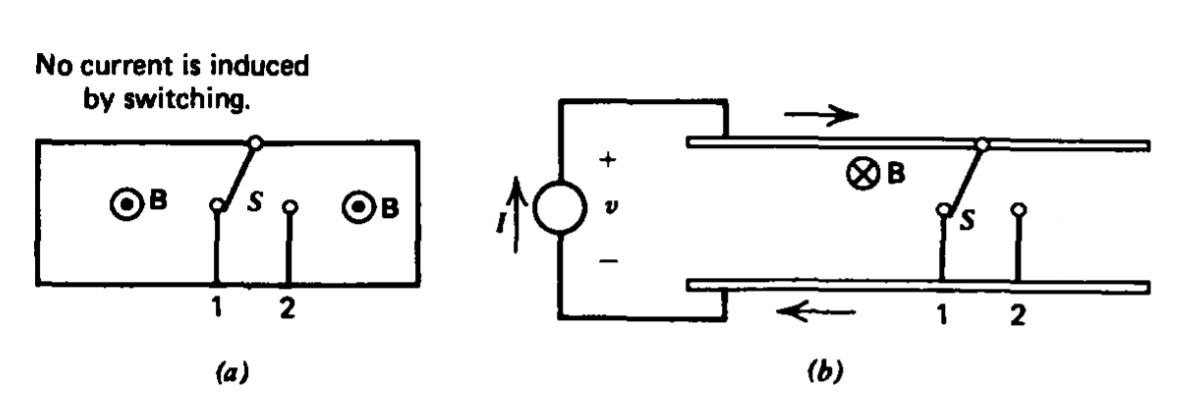
(b) Changes in Magnetic Flux Due to Switching

Changing the configuration of a circuit using a switch does not result in an electromotive force unless the magnetic flux itself changes.

In Figure 6-23a, the magnetic field through the loop is externally imposed and is independent of the switch position. Moving the switch does not induce an EMF because the magnetic flux through any surface remains unchanged.

In Figure 6-23b, a dc current source is connected to a circuit through a switch S. If the switch is instantaneously moved from contact 1 to contact 2, the magnetic field due to the source current I changes. The flux through any fixed area has thus changed resulting in an EMF.

(c) Time Varying Number of Turns on a Coil**

If the number of turns on a coil is changing with time, as in Figure 6-24, the voltage is equal to the time rate of change of flux through the coil. Is the voltage then

\[v \overset{?}{=} N \frac{d \Phi}{dt} \]

or

\[ v \overset{?}{=} \frac{d}{d t}(N \Phi)=N \frac{d \Phi}{d t}+\Phi \frac{d N}{d t} \]

Figure 6-23 (a) Changes in a circuit through the use of a switch does not by itself generate an EMF. (b) However, an EMF can be generated if the switch changes the magnetic field.

Figure 6-24 (a) If the number of turns on a coil is changing with time, the induced voltage is \(v = N(t) d \Phi /dt \). A constant flux does not generate any voltage. (b) If the flux itself is proportional to the number of turns, a dc current can generate a voltage. (c) With the tap changing coil, the number of turns per unit length remains constant so that a dc current generates no voltage because the flux does not change with time.

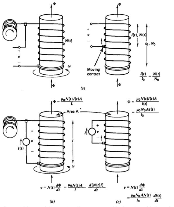
For the first case a dc flux generates no voltage while the second does.

We use Faraday's law with a stationary contour instantaneously within the wire. Because the contour is stationary, its area of NA is not changing with time and so can be taken outside the time derivative in the flux term of Faraday's law so that the voltage is given by (52) and (53) is wrong. Note that there is no speed voltage contribution in the electromotive force because the velocity of the wire is in the same direction as the contour (\(\textbf{v} \times \textbf{B} \cdot \textbf{dl} = 0\)).

If the flux (\(\Phi\) itself depends on the number of turns, as in Figure 6-24b, there may be a contribution to the voltage even if the exciting current is dc. This is true for the turns being wound onto the cylinder in Figure 6-24b. For the tap changing configuration in Figure 6-24c, with uniformly wound turns, the ratio of turns to effective length is constant so that a dc current will still not generate a voltage.

* H. Sohon, Electrical Essays for Recreation. Electrical Engineering, May (1946), p. 294.

** L. V. Bewley. Flux Linkages and Electromagnetic Induction. Macmillan, New York, 1952.