6.4: The Energy Method for Forces

If the current distribution is known, the magnetic field can be directly found from the Biot-Savart or Ampere's laws. However, when the magnetic field varies with time, the generated electric field within an Ohmic conductor induces further currents that also contribute to the magnetic field.

6-4-1 Resistor-Inductor Model

A thin conducting shell of radius \(R_{i}\) thickness \(\Delta\), and depth \(l\) is placed within a larger conducting cylinder, as shown in Figure 6-25. A step current \(I_{0}\) is applied at t =0 to the larger cylinder, generating a surface current \(\textbf{K} = (I_{0}/l) \textbf{i}_{\phi}\). If the length \(l\) is much greater than the outer radius \(R_{0}\), the magnetic field is zero outside the cylinder and uniform inside for \(R_{i} < r < R_{0}\). Then from the boundary condition on the discontinuity of tangential H given in Section 5-6-1, we have

\[\textbf{H}_{0} = \dfrac{I_{0}}{l} \textbf{i}_{z}, \: \: \: \: R_{i} < r < R_{0} \]

The magnetic field is different inside the conducting shell because of the induced current, which from Lenz's law, flows in the opposite direction to the applied current. Because the shell is assumed to be very thin (\(\Delta << R_{1}\)), this induced current can be considered a surface current related to the volume current and electric field in the conductor as

\[K_{\phi} = J_{\phi} \Delta = (\sigma \Delta) E_{\phi} \]

The product (\(\sigma \Delta\)) is called the surface conductivity. Then the magnetic fields on either side of the thin shell are also related by the boundary condition of Section 5-6-1:

\[H_{i} - H_{0} = K_{\phi} = (\sigma \Delta) E_{\phi} \]

Figure 6-25 A step change in magnetic field causes the induced current within an Ohmic conductor to flow in the direction where its self-flux opposes the externally imposed flux. Ohmic dissipation causes the induced current to exponentially decay with time with a \(L/R\) time constant.

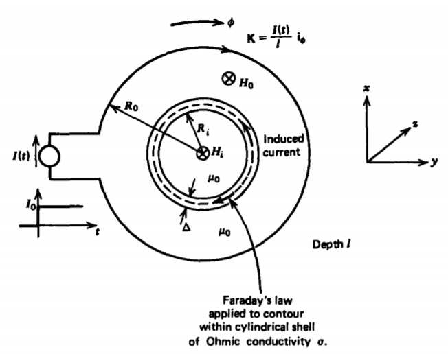
Applying Faraday's law to a contour within the conducting shell yields

\[\oint_{L} \textbf{E} \cdot \textbf{dl} = - \dfrac{d}{dt} \int_{S} \textbf{B} \cdot \textbf{dS} \Rightarrow E_{\phi} 2 \pi R_{i} = - \mu_{0} \pi R^{2}_{i} \dfrac{dH_{i}}{dt} \]

where only the magnetic flux due to \(H_{i}\) passes through the contour. Then using (1)-(3) in (4) yields a single equation in \(H_{i}\):

\[\dfrac{dH_{i}}{dt} + \dfrac{H_{i}}{\tau} = \dfrac{I(t)}{l \tau}, \: \: \: \: \tau = \dfrac{\mu_{0} R_{i} \sigma \Delta}{2} \]

where we recognize the time constant \(\tau\) as just being the ratio of the shell's self-inductance to resistance:

\[: = \dfrac{\Phi}{K_{\phi}l} = \dfrac{\mu_{0} \pi R^{2}_{i}}{l}, \: \: \: \: R = \dfrac{2 \pi R_{i}}{\sigma l \Delta}, \: \: \: \: \tau = \dfrac{L}{R} = \dfrac{\mu_{0}R_{i} \sigma \Delta}{2} \]

The solution to (5) for a step current with zero initial magnetic field is

\[H_{i} = \dfrac{I_{0}}{l}(1 - e^{-t/tau}) \]

Initially, the magnetic field is excluded from inside the conducting shell by the induced current. However, Ohmic dissipation causes the induced current to decay with time so that the magnetic field may penetrate through the shell with characteristic time constant \(\tau\).

* Much of the treatment of this section is similar to that of H. H. Woodson and J. R. Melcher, Electromechanical Dynamics, PartII, Wiley, N. Y., 1968, Ch. 7.

6-4-2 The Magnetic Diffusion Equation

The transient solution for a thin conducting shell could be solved using the integral laws because the geometry constrained the induced current to flow azimuthally with no radial variations. If the current density is not directly known, it becomes necessary to self-consistently solve for the current density with the electric and magnetic fields:

\[\nabla \times \textbf{E} = - \dfrac{\partial \textbf{B}}{\partial t} \: \textrm{(Faraday's law)} \]

\[ \nabla \times \textbf{H} = \textbf{J}_{f} \: \textrm{(Ampere's law)} \]

\[ \nabla \cdot \textbf{B} = 0 \: \textrm{(Gauss's law)} \]

For linear magnetic materials with constant permeability \(\mu\) and constant Ohmic conductivity \(\sigma\) moving with velocity U, the constitutive laws are

\[\textbf{B} = \mu \textbf{J}, \: \: \: \: \textbf{J}_{f} = \sigma (\textbf{E} + \textbf{U} \times \mu \textbf{H}) \]

We can reduce (8)-(11) to a single equation in the magnetic field by taking the curl of (9), using (8) and (11) as

\[\nabla \times (\nabla \times \textbf{H}) = \nabla \times \textbf{J}_{f} \\ = \sigma [ \nabla \times \textbf{E} + \mu \nabla \times (\textbf{U} \times \textbf{H})] \\ = \mu \sigma \bigg( - \dfrac{\partial \textbf{H}}{\partial t} + \nabla \times (\textbf{U} \times \textbf{H}) \bigg) \]

The double cross product of H can be simplified using the vector identity

\[\nabla \times (\nabla \times \textbf{H}) = \nabla (\nabla \cancelto{0}{\cdot} \textbf{H}) - \nabla^{2} \textbf{H} \\ \Rightarrow \dfrac{1}{\mu \sigma} \nabla^{2} \textbf{H} = \dfrac{\partial \textbf{H}}{\partial t} - \nabla \times (\textbf{U} \times \textbf{H}) \]

where H has no divergence from (10). Remember that the Laplacian operator on the left-hand side of (13) also differentiates the directionally dependent unit vectors in cylindrical (\(\textbf{i}_{\textrm{r}}\) and \(\textbf{i}_{\phi}\)) and spherical (\(\textbf{i}_{r}, \: \textbf{i}_{\theta},\) and \(\textbf{i}_{\phi}\)) coordinates.

6-4-3 Transient Solution with No Motion (U =0)

A step current is turned on at t =0, in the parallel plate geometry shown in Figure 6-26. By the right-hand rule and with the neglect of fringing, the magnetic field is in the z direction and only depends on the x coordinate, \(B_{z} (x,t)\), so that (13) reduces to

\[\dfrac{\partial^{2}H_{z}}{\partial x^{2}} - \sigma \mu \dfrac{\partial H_{z}}{\partial t} = 0 \]

which is similar in form to the diffusion equation of a distributed resistive-capacitive cable developed in Section 3-6-4.

In the dc steady state, the second term is zero so that the solution in each region is of the form

\[\dfrac{\partial^{2}H_{z}}{\partial x^{2}} = 0 \Rightarrow H_{z} = ax + b \]

Figure 6-26 (a) A current source is instantaneously turned on at t =0. The resulting magnetic field within the Ohmic conductor remains continuous and is thus zero at t = 0 requiring a surface current at x =0. (b) For later times the magnetic field and current diffuse into the conductor with longest time constant \(\tau = \sigma \mu d^{2}/\pi^{2}\) towards a steady state of uniform current with a linear magnetic field.

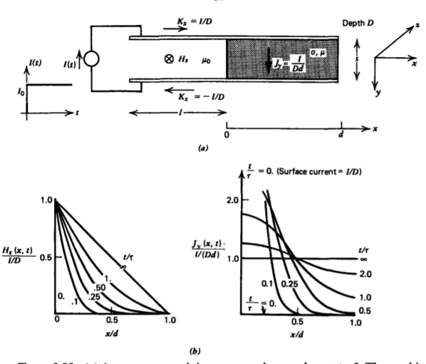
where a and b are found from the boundary conditions. The current on the electrodes immediately spreads out to a uniform surface distribution \(\pm (I/D) \textbf{i}_{x}\), traveling from the upper to lower electrode uniformly through the Ohmic conductor. Then, the magnetic field is uniform in the free space region, decreasing linearly to zero within the Ohmic conductor being continuous across the interface at x =0:

\[\lim_{t \rightarrow \infty} H_{z} (x) = \left \{ \begin{matrix} \dfrac{I}{D}, \: \: \: \: -l \leq x \leq 0 \\ \dfrac{I}{Dd} (d-x), & 0 \leq x \leq d \end{matrix} \right. \]

In the free space region where \(\sigma = 0\), the magnetic field remains constant for all time. Within the conducting slab, there is an initial charging transient as the magnetic field builds up to the linear steady-state distribution in (16). Because (14) is a linear equation, for the total solution of the magnetic field as a function of time and space, we use superposition and guess a solution that is the sum of the steadystate solution in (16) and a transient solution which dies off with time:

\[H_{z} (x,t) = \dfrac{I}{Dd}(d-x) + \hat{H} (x) e^{-\alpha t} \]

We follow the same procedures as for the lossy cable in Section 3-6-4. At this point we do not know the function \(\hat{H}(x)\) or the parameter \(\alpha\). Substituting the assumed solution of (17) back into (14) yields the ordinary differential equation

\[\dfrac{d^{2} \hat{H}(x)}{dx^{2}} + \sigma \mu \alpha \hat{H} (x) = 0 \]

which has the trigonometric solutions

\[\hat{H}(x) = A_{1} sin \sqrt{\sigma \mu \alpha} x + A_{2} \cos \sqrt{\sigma \mu \alpha} x \]

Since the time-independent part in (17) already meets the boundary conditions of

\[H_{z}(x=0) = I/D \\ H_{z} (x=d) =0 \]

the transient part of the solution must be zero at the ends

\[\hat{H}(x=0) = 0 \Rightarrow A_{2} = 0 \\ \hat{H}(x=d) = 0 \Rightarrow \sin \sqrt{\sigma \mu \alpha} d =0 \]

which yields the allowed values of \(\alpha\) as

\[\sqrt{\sigma \mu \alpha} d = n \pi \Rightarrow \alpha_{n} = \dfrac{1}{\mu \sigma} \bigg( \dfrac{n \pi}{d} \bigg)^{2}, \: \: \: \: n = 1,2,3... \]

Since there are an infinite number of allowed values of \(\alpha\), the most general solution is the superposition of all allowed solutions:

\[H_{z} (x,t) = \dfrac{I}{Dd} (d - x) + \sum_{n=1}^{\infty} A_{n} \sin \dfrac{n \pi x}{d} e^{- \alpha_{n}t} \]

This relation satisfies the boundary conditions but not the initial conditions at t = 0 when the current is first turned on. Before the current takes its step at t =0, the magnetic field is zero in the slab. Right after the current is turned on, the magnetic field must remain zero. Faraday's law would otherwise make the electric field and thus the current density infinite within the slab, which is nonphysical. Thus we impose the initial condition

\[H_{z} (x,t = 0) = 0 = \dfrac{I}{Dd} (d-x) + \sum_{n=1}^{\infty} A_{n} \sin \dfrac{n \pi x}{d} \]

which will allow us to solve for the amplitudes \(A_{n}\) by multiplying (24) through by sin (\(m \pi x/d\)) and then integrating over x from 0 to d:

\[0 = \dfrac{I}{Dd} \int_{0}^{d} (d-x) \sin \dfrac{m \pi x}{d} dx + \sum_{n=1}^{\infty} A_{n} \int_{0}^{d} \sin \dfrac{n \pi x}{d} \sin \dfrac{m \pi x}{d} dx \]

The first term on the right-hand side is easily integrable* while the product of sine terms integrates to zero unless m = n, yielding

\[A_{m} = - \dfrac{2I}{m \pi D} \]

The total solution is thus

\[H_{z} (x,t) = \dfrac{I}{D} \bigg(1 - \dfrac{x}{d} - 2 \sum_{n=1}^{\infty} \dfrac{\sin (n \pi x/d)}{n \pi} e^{-n^{2} t/\tau} \bigg) \]

where we define the fundamental continuum magnetic diffusion time constant \(\tau\) as

\[\tau = \dfrac{1}{\alpha_{1}} = \dfrac{\mu \sigma d^{2}}{\pi^{2}} \]

analogous to the lumped parameter time constant of (5) and (6).

The magnetic field approaches the steady state in times long compared to \(\tau\). For a perfect conductor (\(\sigma \rightarrow \infty\)), this time is infinite and the magnetic field is forever excluded from the slab. The current then flows only along the x = 0 surface. However, even for copper (\(\sigma \approx 6 \times 10^{7}\) siemens/m) 10-cm thick, the time constant is \(\tau \approx \80\) msec, which is fast for many applications. The current then diffuses into the conductor where the current density is easily obtained from Ampere's law as

\[\]\[\begin{align*}  \textbf{J}_{f} &= \nabla \times \textbf{H} \\[4pt] &= - \dfrac{\partial H_{z}}{\partial x} \textbf{i}_{y} \\[4pt] &= \dfrac{I}{Dd} \bigg( 1 + 2 \sum_{n=1}^{\infty} \cos \dfrac{n \pi x}{d} e^{n^{2} t/\tau} \bigg) \textbf{i}_{y} \end{align*} \]

The diffusion of the magnetic field and current density are plotted in Figure 6-26b for various times

The force on the conducting slab is due to the Lorentz force tending to expand the loop and a magnetization force due to the difference of permeability of the slab and the surrounding free space as derived in Section 5-8-1:

\[ \] \[\begin{align*} \textbf{F} &= \mu_{0} (\textbf{M} \cdot \nabla) \textbf{H} + \mu_{0} \textbf{J}_{f} \times \textbf{H} \\[4pt] &= ( \mu - \mu_{0})(\textbf{H} \cdot \nabla) \textbf{H} + \mu_{0} \textbf{J}_{f} \times \textbf{H} \end{align*} \]

For our case with \(\textbf{H} = H_{z} (x) \textbf{i}_{z}\), the magnetization force density has no contribution so that (30) reduces to

\[ \] \[\begin{align*} \textbf{F} &= \mu_{0} (\nabla \times \textbf{H}) \times \textbf{H} \\[4pt] &= \mu_{0} (\textbf{H} \cdot \nabla ) \textbf{H} - \nabla (\dfrac{1}{2} \mu_{0} \textbf{H} \cdot \textbf{H}) \\[4pt] &= - \dfrac{d}{dx} (\dfrac{1}{2} \mu_{0} H^{2}_{z}) \textbf{i}_{x} \end{align*} \]

Integrating (31) over the slab volume with the magnetic field independent of y and z,

\[ \] \[\begin{align*} f_{x} &= - \int_{0}^{d} s D \dfrac{d}{dx} \left(\dfrac{1}{2} \mu_{0}H_{z}^{2}\right) dx \\[4pt] &= - \dfrac{1}{2} \mu_{0} H_{z}^{2} s D \big|_{0}^{d} \\[4pt] &= \dfrac{1}{2} \dfrac{\mu_{0} I^{2}s}{D} \end{align*} \]

gives us a constant force with time that is independent of the permeability. Note that our approach of expressing the current density in terms of the magnetic field in (31) was easier than multiplying the infinite series of (27) and (29), as the result then only depended on the magnetic field at the boundaries that are known from the boundary conditions of (20). The resulting integration in (32) was easy because the force density in (31) was expressed as a pure derivative of x.

6-4-4 The Sinusoidal Steady State (Skin Depth)

We now place an infinitely thick conducting slab a distance d above a sinusoidally varying current sheet \(K_{0} \cos \omega t \textbf{i}_{y}\), which lies on top of a perfect conductor, as in Figure 6-27a. The

Figure 6-27 (a) A stationary conductor lies above a sinusoidal surface current placed upon a perfect conductor so that H =0 for \(x < -d\). (b) The magnetic field and current density propagates and decays into the conductor with the same characteristic length given by the skin depth \(\delta = \sqrt{2/(\omega \mu \sigma)} \) The phase speed of the wave is \(\omega \delta\).

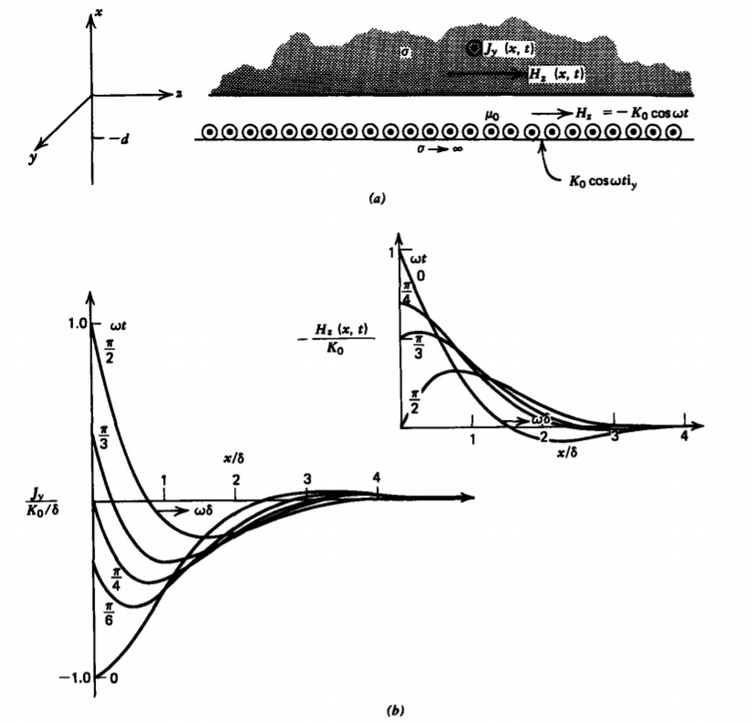
magnetic field within the conductor is then also sinusoidally varying with time:

\[H_{z} (x,t) \textrm{Re} [ \hat{H}_{z} (x) e^{j \omega t} ] \]

Substituting (33) into (14) yields

\[\dfrac{d^{2} \hat{H}_{z}}{dx^{2}} - j \omega \mu \sigma \hat{H}_{z} = 0 \]

with solution

\[\hat{H}_{z} (x) = A_{1} e^{(1 + j)x/\delta} + A_{2} e^{-(1 + j) x/\delta} \]

where the skin depth \(\delta\) is defined as

\[\delta = \sqrt{2/(\omega \mu \sigma)} \]

Since the magnetic field must remain finite far from the current sheet, \(A_{1}\) must be zero. The magnetic field is also continuous across the x =0 boundary because there is no surface current, so that the solution is

\[H_{z} (x,t) = \textrm{Re} [- K_{0} e^{-(1 + j) x/\delta} e^{j \omega t} ] \\ = - K_{0} \cos (\omega t - x/\delta) e^{-x/\delta}, \: \: \: x \geq 0 \]

where the magnetic field in the gap is uniform, determined by the discontinuity in tangential H at \(x = -d\) to be \(H_{z} = -K_{y}\) for \(-d < x \leq 0\) since within the perfect conductor \((x < -d \textbf{H} = 0\). The magnetic field diffuses into the conductor as a strongly damped propagating wave with characteristic penetration depth \(\delta\). The skin depth \(\delta\) is also equal to the propagating wavelength, as drawn in Figure 6-27b. The current density within the conductor

\[\text{J}_{f} = \nabla \times \textbf{H} = - \dfrac{\partial H_{z}}{\partial x} \textbf{i}_{y} \\ = + \dfrac{K_{0} e^{-x/\delta}}{\delta} \bigg[ \sin \bigg( \omega t - \dfrac{x}{\delta} \bigg) - \cos \bigg( \omega t - \dfrac{x}{\delta} \bigg) \bigg] \textbf{i}_{y} \]

is also drawn in Figure 6-27b at various times in the cycle, being confined near the interface to a depth on the order of \(\delta\). For a perfect conductor, \(\delta \rightarrow 0\), and the volume current becomes a surface current.

Seawater has a conductivity of \( \approx 4\) siemens/m so that at a frequency of \(f\) = 1 MHz (\( \omega = 2 \pi f\)) the skin depth is \( \delta \approx 0.25\). This is why radio communications to submarines are difficult. The conductivity of copper is \(\sigma \approx 6 \times 10^{7}\) siemens/m so that at 60 Hz the skin depth is \(\delta \approx 8\) mm. Power cables with larger radii have most of the current confined near the surface so that the center core carries very little current. This reduces the cross-sectional area through which the current flows, raising the cable resistance leading to larger power dissipation.

Again, the magnetization force density has no contribution to the force density since \(H_{z}\) only depends on x:

\[\textbf{F} = \mu_{0} (\textbf{M} \cdot \nabla) \textbf{H} + \mu_{0} \textbf{J}_{f} \times \textbf{H}\\ = \mu_{0} (\nabla \times \textbf{H}) \times \textbf{H} \\ = - \nabla (\dfrac{1}{2} \mu_{0} \textbf{H} \cdot \textbf{H}) \]

The total force per unit area on the slab obtained by integrating (39) over x depends only on the magnetic field at x = 0:

\[f_{x} = - \int_{0}^{\infty} \dfrac{d}{dx} \bigg( \dfrac{\mu_{0}}{2} H_{z}^{2} \bigg) dx \\ = - \dfrac{1}{2} \mu_{0} H_{z}^{2} \big|_{0}^{\infty} \\ = \dfrac{1}{2} \mu_{)} K_{0}^{2} \cos^{2} \omega t \]

because again H is independent of y and z and the x component of the force density of (39) was written as a pure derivative with respect to x. Note that this approach was easier than integrating the cross product of (38) with (37).

This force can be used to levitate the conductor. Note that the region for \(x > \delta\) is dead weight, as it contributes very little to the magnetic force.

* \(\int_{0}^{d} (d-x) \sin \dfrac{m \pi x}{d} dx = \dfrac{d^{2}}{m \pi}\)

6-4-5 Effects of Convection

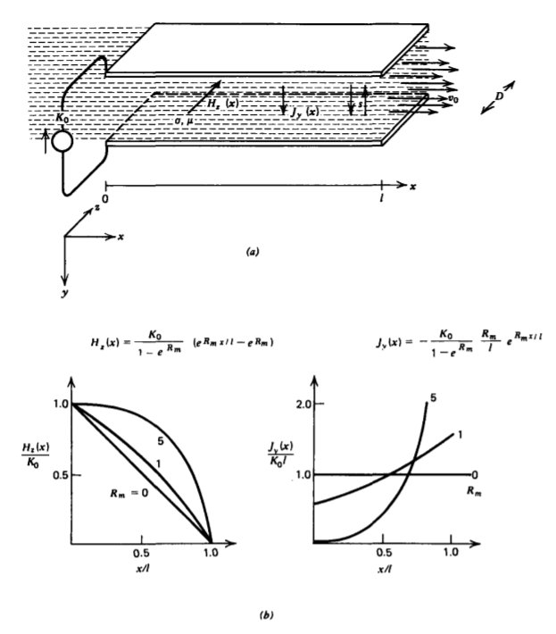
A distributed dc surface current \(-K_{0} \textbf{i}_{y}\) at x =0 flows along parallel electrodes and returns via a conducting fluid moving to the right with constant velocity \(v_{0} \textbf{i}_{x}\), as shown in Figure 6-28a. The flow is not impeded by the current source at x = 0. With the neglect of fringing, the magnetic field is purely z directed and only depends on the x coordinate, so that (13) in the dc steady state, with \(\textbf{U} = v_{0} \textbf{i}_{x}\) being a constant, becomes*

\[\dfrac{d^{2}H_{z}}{dx^{2}} - \mu \sigma v_{0} \dfrac{dH_{z}}{dx} = 0 \]

Solutions of the form

\[H_{z} (x) = A e^{px} \]

Figure 6-28 (a) A conducting material moving through a magnetic field tends to pull the magnetic field and current density with it. (b) The magnetic field and current density are greatly disturbed by the flow when the magnetic Reynolds number is large, \(R_{m} = \sigma \mu Ul >>1\).

when substituted back into (41) yield two allowed values of p,

\[p^{2} - \mu \sigma v_{0} p = 0 \Rightarrow p = 0, \: \: \: \: p = \mu \sigma v_{0} \]

Since (41) is linear, the most general solution is just the sum of the two allowed solutions,

\[H_{z} (x) = A_{1} e^{R_{m} x/l} + A_{2} \]

where the magnetic Reynold's number is defined as

\[R_{m} = \sigma \mu v_{0} l = \dfrac{\sigma \mu l^{2}}{l/v_{0}} \]

and represents the ratio of a representative magnetic diffusion time given by (28) to a fluid transport time (\(l/v_{0}\)). The boundary conditions are

\[H_{z} (x=0) = K_{0}, \: \: \: \: H_{z}(x=l) = 0 \]

so that the solution is

\[H_{z} (x) = \dfrac{K_{0}}{1-e^{R_{m}}} (e^{R_{m}x/l} - e^{R_{m}}) \]

The associated current distribution is then

\[\textbf{J}_{f} = \nabla \times \textbf{H} = - \dfrac{\partial H_{z}}{\partial x} \textbf{i}_{y} \\ = - \dfrac{K_{0}}{1-e^{R_{m}}} \dfrac{R_{m}}{l} e^{R_{m}x/l} \textbf{i}_{y} \]

The field and current distributions plotted in Figure 6-28b for various \(R_{m}\) show that the magnetic field and current are pulled along in the direction of flow. For small \(R_{m}\) the magnetic field is hardly disturbed from the zero flow solution of a linear field and constant current distribution. For very large \(R_{m} >> 1\), the magnetic field approaches a uniform distribution while the current density approaches a surface current at \(x = l\).

The force on the moving fluid is independent of the flow velocity:

\[\textbf{f} = \int_{0}^{l} \textbf{J} \times \mu_{0} \textbf{H} s D \: dx \\ = - \dfrac{K_{0}^{2}}{(1 - e^{R_{m}})^{2}} \mu_{0} \dfrac{R_{m}}{l} sD \int_{0}^{l} e^{R_{m}x/l}(e^{R_{m}x/l}-e^{R_{m}}) dx \: \textbf{i}_{x} \\ = - \dfrac{K_{0}^{2} \mu_{0} sD}{(1-e^{R_{m}})^{2}} e^{R_{m}x/l} \bigg( \dfrac{e^{R_{m}x/l}}{2} - e^{R_{m}} \bigg) \bigg|_{0}^{l} \textbf{i}_{x} \\ = \dfrac{1}{2} \mu_{0} K_{0}^{2} s D \textbf{i}_{x} \]

*\(\nabla \times (\textbf{U} \times \textbf{H}) = \textbf{U} (\nabla \cancelto{0}{\cdot} \textbf{H}) - \textbf{H}(\nabla \cancelto{0}{\cdot} \textbf{U}) + (\textbf{H} \cancelto{0}{\cdot} \nabla) \textbf{U} - (\textbf{U} \cdot \nabla) \textbf{H} = - v_{0} \dfrac{d \textbf{H}}{dx}\)

6-4-6 A Linear Induction Machine

The induced currents in a conductor due to a time varying magnetic field give rise to a force that can cause the conductor to move. This describes a motor. The inverse effect is when we cause a conductor to move through a time varying magnetic field generating a current, which describes a generator.

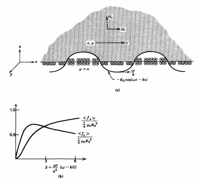
The linear induction machine shown in Figure 6-29a assumes a conductor moves to the right at constant velocity \(U \textbf{i}_{z}\). Directly below the conductor with no gap is a surface current placed on top of an infinitely permeable medium

\[\textbf{K} (t) = -K_{0} \cos (\omega t- kz) \textbf{i}_{y} = \textrm{Re} [ - K_{0} e^{j(\omega t - kz)} \textbf{i}_{y}] \]

which is a traveling wave moving to the right at speed \(\omega /k\). For x >0, the magnetic field will then have x and z components of the form

\[H_{z}(x, z, t) = \textrm{Re} [ \hat{H}_{z} (x) e^{j (\omega t- kz)}] \\ H_{x} (x, z, t) = \textrm{Re} [\hat{H}_{x} (x) e^{j(\omega t - kz)}] \]

Figure 6-29 (a) A traveling wave of surface current induces currents in a conductor that is moving at a velocity U different from the wave speed \(\omega/k\). (b) The resulting forces can levitate and propel the conductor as a function of the slip S, which measures the difference in speeds of the conductor and traveling wave.

where (10) (\(\nabla \cdot \textbf{B} = 0\)) requires these components to be related as

\[\dfrac{d \hat{H}_{x}}{dx} - jk \hat{H}_{z} =0 \]

The z component of the magnetic diffusion equation of (13) is

\[\dfrac{d^{2} \hat{H}_{z}}{d x^{2}} - k^{2} \hat{H}_{2} = j \mu \sigma (\omega - k U) \hat{H}_{z} \]

which can also be written as

\[\dfrac{d^{2}\hat{H}_{z}}{dx^{2}} - \gamma^{2} \hat{H}_{z} =0 \]

where

\[\gamma^{2} = k^{2} (1 + jS), \: \: \: \: S = \dfrac{\mu \sigma}{k^{2}} (\omega - kU) \]

and S is known as the slip. Solutions of (54) are again exponential but complex because \(\gamma\) is complex:

\[\hat{H}_{z} = A_{1} e^{\gamma x} + A_{2} e^{-\gamma x} \]

Because \(\hat{H}_{z}\) must remain finite far from the current sheet, \(A_{1} = 0\), so that using (52) the magnetic field is of the form

\[\hat{\textbf{H}} = K_{0} e^{- \gamma x} \bigg( \textbf{i}_{z} - \dfrac{jk}{\gamma} \textbf{i}_{x} \bigg) \]

where we use the fact that the tangential component of H is discontinuous in the surface current, with H = 0 for x<0.

The current density in the conductor is

\[\textbf{J}_{f} = \nabla \times \textbf{H} = \textbf{i}_{y} \bigg( \dfrac{\partial H_{x}}{\partial z} - \dfrac{\partial H_{z}}{\partial x} \bigg) \Rightarrow \hat{J}_{y} = -jk \hat{H}_{x} - \dfrac{d \hat{H}_{z}}{dx} \\ = K_{0} e^{- \gamma x} \dfrac{(\gamma^{2} - k^{2})}{\gamma} \\ = \dfrac{K_{0}k^{2}jS e^{-\gamma x}}{\gamma} \]

If the conductor and current wave travel at the same speed (\(\omega/k = U\)), no current is induced as the slip is zero. Currents are only induced if the conductor and wave travel at different velocities. This is the principle of all induction machines.

The force per unit area on the-conductor then has x and z components:

\[\textbf{f} = \int_{0}^{\infty} \textbf{J} \times \mu_{0} \textbf{H} dx \\ = \int_{0}^{\infty} \mu_{0} J_{y} (H_{z} \textbf{i}_{x} - H_{x} \textbf{i}_{z}) dx \]

These integrations are straightforward but lengthy because first the instantaneous field and current density must be found from (51) by taking the real parts. More important is the time-average force per unit area over a period of excitation

\[< \textbf{f} > = \dfrac{\omega}{2 \pi} \int_{0}^{2 \pi/ \omega} \textbf{f} dt \]

Since the real part of a complex quantity is equal to half the sum of the quantity and its complex conjugate,

\[A = \textrm{Re}[\hat{A} e^{j \omega t}] = \dfrac{1}{2} (\hat{A} e^{j \omega t} + \hat{A}* e^{-j \omega t}) \\ B = \textrm{Re} [\hat{B} e^{j \omega t}] = \dfrac{1}{2} (\hat{B} e^{j \omega t} + \hat{B}* e^{-j \omega t}) \]

the time-average product of two quantities is

\[\dfrac{\omega}{2 \pi} \int_{0}^{2 \pi/\omega} AB dt = \dfrac{1}{4} \dfrac{\omega}{2 \pi} \int_{0}^{2 \pi/\omega} (\hat{A} \hat{B} e^{2 j \omega t} + \hat{A} * \hat{B} + \hat{A} \hat{B} * \\ + \hat{A} * \hat{B}* e^{-2 j \omega t}) dt \\ = \dfrac{1}{4} (\hat{A} * \hat{B} + \hat{A} \hat{B} *) \\ \hat{1}{2} \textrm{Re} (\hat{A} \hat{B} *) \]

which is a formula often used for the time-average power in circuits where A and B are the voltage and current.

Then using (62) in (59), the x component of the time-average force per unit area is

\[ <f_{x}> = \dfrac{1}{2} \textrm{Re} \bigg( \int_{0}^{\infty} \mu_{0} \hat{J}_{y} \hat{H}_{z} * dx \bigg) \\ = \dfrac{\mu_{0}}{2} K_{0}^{2} k^{2} S \textrm{Re} \bigg( \dfrac{j}{\gamma} \int_{0}^{\infty} e^{- (\gamma + \gamma * ) x} dx \bigg) \\ = \dfrac{\mu_{0}}{2} K_{0}^{2} k^{2} S \textrm{Re} \bigg( \dfrac{j}{\gamma (\gamma + \gamma *)} \bigg) \\ = \dfrac{1}{4} \dfrac{\mu_{0}K_{0}^{2}S^{2}}{[1 + S^{2} + (1 + S^{2})^{1/2}]} = \dfrac{1}{4} \mu_{0}K_{0}^{2} \bigg( \dfrac{\sqrt{1 + S^{2}} -1}{\sqrt{1 + S^{2}}} \bigg) \]

where the last equalities were evaluated in terms of the slip S from (55).

We similarly compute the time-average shear force per unit area as

\[< f_{z} > = - \dfrac{1}{2} \textrm{Re} \bigg( \int_{0}^{\infty} \mu_{0} J_{y} H*_{x} dx \bigg) \\ = \dfrac{\mu_{0}}{2} \dfrac{K_{0}^{2} k^{3} S}{\gamma \gamma*} \textrm{Re} \bigg( \int_{0}^{\infty} e^{- (\gamma + \gamma*)x} dx \bigg) \\ = \dfrac{\mu_{0}}{2} \dfrac{k^{3} K_{0}^{2}S}{\gamma \gamma*} \textrm{Re} \bigg( \dfrac{1}{(\gamma + \gamma*)} \bigg) \\ = \dfrac{\mu_{0}K_{0}^{2}S}{4 \sqrt{1 + S^{2}} \textrm{Re} ( \sqrt{1 + jS})} \]

When the wave speed exceeds the conductor's speed (\(\omega/k > U\)), the force is positive as S>0 so that the wave pulls the conductor along. When S < 0, the slow wave tends to pull the conductor back as \(<f_{z}> < 0\). The forces of (63) and (64), plotted in Figure 6-29b, can be used to simultaneously lift and propel a conducting material. There is no force when the wave and conductor travel at the same speed (\(\omega/k = U\)) as the slip is zero (\(S = 0\)). For large S, the levitating force \(<f_{x}>\) approaches the constant value \(\dfrac{1}{4} \mu_{0}K_{0}^{2}\) while the shear force approaches zero. There is an optimum value of S that maximizes \(< f_{z}>\). For smaller S, less current is induced while for larger S the phase difference between the imposed and induced currents tend to decrease the time-average force.

6-4-7 Superconductors

In the limit of infinite Ohmic conductivity (\(\sigma \rightarrow \infty\)), the diffusion time constant of (28) becomes infinite while the skin depth of (36) becomes zero. The magnetic field cannot penetrate a perfect conductor and currents are completely confined to the surface.

However, in this limit the Ohmic conduction law is no longer valid and we should use the superconducting constitutive law developed in Section 3-2-2d for a single charge carrier:

\[\dfrac{\partial \textbf{J}}{\partial t} = \omega_{p}^{2} \varepsilon \textbf{E} \]

Then for a stationary medium, following the same procedure as in (12) and (13) with the constitutive law of (65), (8)-(11) reduce to

\[ \nabla^2 \frac{\partial \mathbf{H}}{\partial t}-\omega_p^2 \varepsilon \mu \frac{\partial \mathbf{H}}{\partial t}=0 \Rightarrow \nabla^2\left(\mathbf{H}-\mathbf{H}_0\right)-\omega_p^2 \varepsilon \mu\left(\mathbf{H}-\mathbf{H}_0\right)=0 \]

where \(\textbf{H}_{0}\) is the instantaneous magnetic field at \(t =0\). If the superconducting material has no initial magnetic field when an excitation is first turned on, then \(\textbf{H}_{0} = 0\).

If the conducting slab in Figure 6-27a becomes superconducting, (66) becomes

\[\dfrac{d^{2}H_{z}}{dx^{2}} - \dfrac{\omega_{p}^{2}}{c^{2}}H_{z} = 0, \: \: \: c = \dfrac{1}{\sqrt{\varepsilon \mu}} \]

where c is the speed of light in the medium.

The solution to (67) is

\[H_{z} = A_{1} e^{\omega_{p} x/c} + A_{2} e^{- \omega_{p} x/c} \\ = - K_{0} \cos \omega t \: e^{-\omega_{0} x/c} \]

where we use the boundary condition of continuity of tangential H at x = 0.

The current density is then

\[J_{y} = - \dfrac{\partial H_{z}}{\partial x} \\ = - \dfrac{K_{0} \omega_{p}}{c} \cos \omega t e^{- \omega_{p} x/c} \]

For any frequency \(\omega\), including dc (\(\omega\) = 0), the field and current decay with characteristic length:

\[l_{c} = c/\omega_{p} \]

Since the plasma frequency \(\omega_{p}\) is typically on the order of 10¹⁵ radian/sec, this characteristic length is very small, \(l_{c} \approx 3 \times 10^{8} / 10^{15} \approx 3 \times 10^{-7}\) m. Except for this thin sheath, the magnetic field is excluded from the superconductor while the volume current is confined to this region near the interface.

There is one experimental exception to the governing equation in (66), known as the Meissner effect. If an ordinary conductor is placed within a dc magnetic field H₀ and then cooled through the transition temperature for superconductivity, the magnetic flux is pushed out except for a thin sheath of width given by (70). This is contrary to (66), which allows the time-independent solution H = H₀, where the magnetic field remains trapped within the superconductor. Although the reason is not well understood, superconductors behave as if H₀ =0 no matter what the initial value of magnetic field.