6.5: Energy Stored in The Magnetic Field

6-5-1 A Single Current Loop

The differential amount of work necessary to overcome the electric and magnetic forces on a charge q moving an incremental distance ds at velocity v is

\[dW_{q} = - q (\textbf{E} + \textbf{v} \times \textbf{B}) \cdot \textbf{ds} \]

(a) Electrical Work

If the charge moves solely under the action of the electrical and magnetic forces with no other forces of mechanical origin, the incremental displacement in a small time dt is related to its velocity as

\[\textbf{ds} = \textbf{v} dt \]

Then the magnetic field cannot contribute to any work on the charge because the magnetic force is perpendicular to the charge's displacement:

\[d W_{q} = - q \textbf{v} \cdot \textbf{E} dt \]

and the work required is entirely due to the electric field. Within a charge neutral wire, the electric field is not due to Coulombic forces but rather arises from Faraday's law. The moving charge constitutes an incremental current element,

\[q \textbf{v} = i \textbf{dl} \Rightarrow d W_{q} = - i \textbf{E} \cdot \textbf{dl} dt \]

so that the total work necessary to move all the charges in the closed wire is just the sum of the work done on each current element,

\[\]\[\begin{align*} dW &= \oint_{L} d W_{q} \\[4pt] &= -i dt \oint_{L} \textbf{E} \cdot \textbf{dl} \\[4pt] &= i dt \frac{d}{dt} \int_{S} \textbf{B} \cdot \textbf{dS} \\[4pt] &= i dt \frac{d \Phi}{dt} \\[4pt] &= i d \Phi \end{align*} \]

which through Faraday's law is proportional to the change of flux through the current loop. This flux may be due to other currents and magnets (mutual flux) as well as the self-flux due to the current \(i\). Note that the third relation in (5) is just equivalent to the circuit definition of electrical power delivered to the loop:

\[p = \frac{dW}{dt} = i \frac{d \Phi}{dt} = vi \]

All of this energy supplied to accelerate the charges in the wire is stored as no energy is dissipated in the lossless loop and no mechanical work is performed if the loop is held stationary.

(b) Mechanical Work

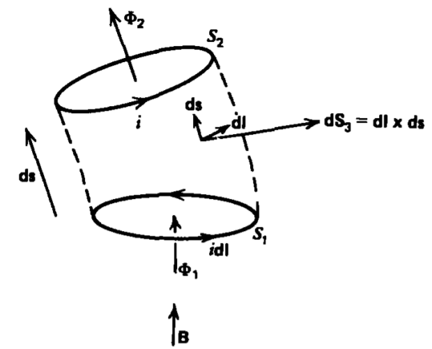
The magnetic field contributed no work in accelerating the charges. This is not true when the current-carrying wire is itself moved a small vector displacement ds requiring us to perform mechanical work,

\[dW = - (i \textbf{dl} \times \textbf{B}) \cdot \textbf{ds} = i (\textbf{B} \times \textbf{dl}) \cdot \textbf{ds} \\ = i \textbf{B} \cdot (\textbf{dl} \times \textbf{ds}) \]

where we were able to interchange the dot and the cross using the scalar triple product identity proved in Problem 1-10a. We define S₁ as the area originally bounding the loop and S₂ as the bounding area after the loop has moved the distance ds, as shown in Figure 6-30. The incremental area dS₃ is then the strip joining the two positions of the loop defined by the bracketed quantity in (7):

\[\textbf{dS_{3}} = \textbf{dl} \times \textbf{ds} \]

The flux through each of the contours is

\[\Phi_{1} = \int_{S_{1}} \textbf{B} \cdot \textbf{dS}, \: \: \: \: \Phi_{2} = \int_{S_{2}} \textbf{B} \cdot \textbf{dS} \]

where their difference is just the flux that passes outward through \(\textbf{dS}_{3}\):

\[d \Phi = \Phi_{1} - \Phi_{2} = \textbf{B} \cdot \textbf{dS}_{3} \]

The incremental mechanical work of (7)-necessary to move the loop is then identical to (5):

\[dW = i \textbf{B} \cdot \textbf{dS}_{3} = i d \Phi \]

Here there was no change of electrical energy input, with the increase of stored energy due entirely to mechanical work in moving the current loop.

Figure 6-30 The mechanical work necessary to move a current-carrying loop is stored as potential energy in the magnetic field.

6-5-2 Energy and Inductance

If the loop is isolated and is within a linear permeable material, the flux is due entirely to the current, related through the self-inductance of the loop as

\[\Phi = Li \]

so that (5) or (11) can be integrated to find the total energy in a loop with final values of current I and flux \(\Phi\):

\[W = \int_{0}^{\Phi} i d \Phi \\ = \int_{0}^{\Phi} \frac{\Phi}{L} d \Phi \\ = \frac{1}{2} \frac{\Phi^{2}}{L} = \frac{1}{2} LI^{2} = \frac{1}{2} I \Phi \]

6-5-3 Current Distributions

The results of (13) are only true for a single current loop. For many interacting current loops or for current distributions, it is convenient to write the flux in terms of the vector potential using Stokes' theorem:

\[\Phi = \int_{S} \textbf{B} \cdot \textbf{dS} = \int_{S} (\nabla \times \textbf{A}) \cdot \textbf{dS} = \oint_{L} \textbf{A} \cdot \textbf{dl} \]

Then each incremental-sized current element carrying a current I with flux \(d \Phi\) has stored energy given by (13):

\[dW = \frac{1}{2} I d \Phi = \frac{1}{2} \textbf{I} \cdot \textbf{A} dl \]

For N current elements, (15) generalizes to

\[W = \frac{1}{2} (\textbf{I}_{1} \cdot \textbf{A}_{1} dl_{1} + \textbf{I}_{2} \cdot \textbf{A}_{2} dl_{2} + ... + \textbf{I}_{N} \cdot \textbf{A}_{N} dl_{N}) \\ = \frac{1}{2} \sum_{n=1}^{N} \textbf{I}_{n} \cdot \textbf{A}_{n} dl_{n} \]

If the current is distributed over a line, surface, or volume, the summation is replaced by integration:

\[W = \left \{ \begin{matrix} \frac{1}{2} \int_{L} \textbf{I}_{f} \cdot \textbf{A} dl & \textrm{(line current)} \\ \frac{1}{2} \int_{S} \textbf{K}_{f} \cdot \textbf{A} d \textrm{S} & \textrm{(surface current)} \\ \frac{1}{2} \int_{\textrm{V}} \textbf{J}_{f} \cdot \textbf{A} d \textrm{V} \textrm{(volume current)} \end{matrix} \right. \]

Remember that in (16) and (17) the currents and vector potentials are all evaluated at their final values as opposed to (11), where the current must be expressed as a function of flux.

6-5-4 Magnetic Energy Density

This stored energy can be thought of as being stored in the magnetic field. Assuming that we have a free volume distribution of current \(\textbf{J}_{f}\) we use (17) with Ampere's law to express \(\textbf{J}_{f}\) in terms of H,

\[W = \frac{1}{2} \int_{\textrm{V}} \textbf{J}_{f} \cdot \textbf{A} d \textrm{V} = \frac{1}{2} \int_{\textrm{V}} (\nabla \times \textbf{H}) \cdot \textbf{A} d \textrm{V} \]

where the volume V is just the volume occupied by the current. Larger volumes (including all space) can be used in (18), for the region outside the current has \(\textbf{J}_{f} = 0\) so that no additional contributions arise.

Using the vector identity

\[\nabla \cdot (\textbf{A} \times \textbf{H}) = \textbf{H} \cdot (\nabla \times \textbf{A}) - \textbf{A} \cdot (\nabla \times \textbf{H}) \\ = \textbf{H} \cdot \textbf{B} - \textbf{A} \cdot (\nabla \times \textbf{H}) \]

we rewrite (18) as

\[W = \frac{1}{2} \int_{\textrm{V}} [ \textbf{H} \cdot \textbf{B} - \nabla \cdot (\textbf{A} \times \textbf{H}) ] d \textrm{V} \]

The second term on the right-hand side can be converted to a surface integral using the divergence theorem:

\[ \int_{\textrm{V}} \nabla \cdot (\textbf{A} \times \textbf{H}) d \textrm{V} = \oint_{S} (\textbf{A} \times \textbf{H}) \cdot \textbf{dS} \]

It now becomes convenient to let the volume extend over all space so that the surface is .at infinity. If the current distribution does not extend to infinity the vector potential dies off at least as \(1/r\) and the magnetic field as \(1/r^{2}\). Then, even though the area increases as \(r^{2}\), the surface integral in (21) decreases at least as \(1/r\) and thus is zero when S is at infinity. Then (20) becomes simply

\[W = \frac{1}{2} \int_{\textrm{V}} \textbf{H} \cdot \textbf{B} d \textrm{V} = \frac{1}{2} \int_{\textrm{V}} \mu H^{2} d \textrm{V} = \frac{1}{2} \int_{\textrm{V}} \frac{B^{2}}{\mu} d \textrm{V} \]

where the volume V now extends over all space. The magnetic energy density is thus

\[\omega = \frac{1}{2} \textbf{H} \cdot \textbf{B} = \frac{1}{2} \mu H^{2} = \frac{1}{2} \frac{B^{2}}{\mu} \]

These results are only true for linear materials where \(\mu\) does not depend on the magnetic field, although it can depend on position.

For a single coil, the total energy in (22) must be identical to (13), which gives us an alternate method to calculating the self-inductance from the magnetic field.

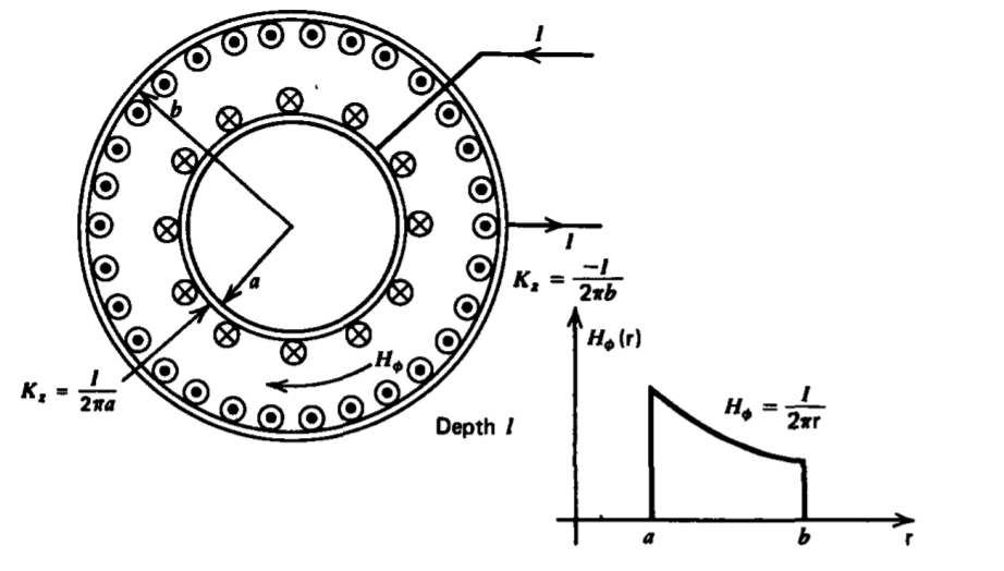
6-5-5 The Coaxial Cable

(a) External Inductance

A typical cable geometry consists of two perfectly conducting cylindrical shells of radii a and b and length \(l\), as shown in Figure 6-31. An imposed current I flows axially as a surface current in opposite directions on each cylinder. We neglect fringing field effects near the ends so that the magnetic field is the same as if the cylinder were infinitely long. Using Ampere's law we find that

\[H_{\phi} = \frac{I}{2 \pi \textrm{r}}, \: \: \: a < \textrm{r} < b \]

The total magnetic flux between the two conductors is

\[\Phi = \int_{a}^{b} \mu_{0} H_{\phi} l d \textrm{r} \\ = \frac{\mu_{0} I l}{2 \pi} \ln \frac{b}{a} \]

giving the self-inductance as

\[L = \frac{\Phi}{I} = \frac{\mu_{0}l}{2 \pi} \ln \frac{b}{a} \]

The same result can just as easily be found by computing the energy stored in the magnetic field

\[W = \frac{1}{2} LI^{2} = \frac{1}{2} \mu_{0} \int_{a}^{b} H^{2}_{\phi} 2 \pi \textrm{r} l d \textrm{r} \\ = \frac{\mu_{0} l I^{2}}{4 \pi} \ln \frac{b}{a} \Rightarrow L = \frac{2 W}{I^{2}} = \frac{\mu_{0} \ln (b/a)}{2 \pi} \]

Figure 6-31 The magnetic field between two current-carrying cylindrical shells forming a coaxial cable is confined to the region between cylinders.

(b) Internal Inductance

If the inner cylinder is now solid, as in Figure 6-32, the current at low enough frequencies where the skin depth is much larger than the radius, is uniformly distributed with density

\[J_{z} = \frac{I}{\pi a^{2}} \]

so that a linearly increasing magnetic field is present within the inner cylinder while the outside magnetic field is

Figure 6-32 At low frequencies the current in a coaxial cable is uniformly distributed over the solid center conductor so that the internal magnetic field increases linearly with radius. The external magnetic field remains unchanged. The inner cylinder can be thought of as many incremental cylindrical shells of thickness dr carrying a fraction of the total current. Each shell links its own self-flux-as well as the mutual flux of the other shells of smaller radius. The additional flux within the current-carrying conductor results in the internal inductance of the cable.

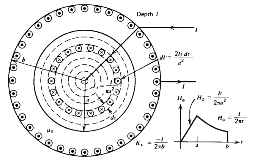
unchanged from (24):

\[H_{\phi} = \left \{ \begin{matrix} \frac{I \textrm{r}}{2 \pi a^{2}}, & 0 < \textrm{r} < a \\ \frac{I}{2 \pi \textrm{r}}, & a < \textrm{r} < b \end{matrix} \right. \]

The self-inductance cannot be found using the flux per unit current definition for a current loop since the current is not restricted to a thin filament. The inner cylinder can be thought of as many incremental cylindrical shells, as in Figure 6-32, each linking its own self-flux as well as the mutual flux of the other shells of smaller radius. Note that each shell is at a different voltage due to the differences in enclosed flux, although the terminal wires that are in a region where the magnetic field is negligible have a well-defined unique voltage difference.

The easiest way to compute the self-inductance as seen by the terminal wires is to use the energy definition of (22):

\[W = \frac{1}{2} \mu_{0} \int_{0}^{b} H^{2}_{\phi} 2 \pi l \textrm{r} d \textrm{r} \\ = \pi l \mu_{0} \bigg[ \int_{0}^{a} \bigg( \frac{I \textrm{r}}{2 \pi a^{2}} \bigg)^{2} \textrm{r} d \textrm{r} + \int_{a}^{b} \bigg( \frac{I}{2 \pi \textrm{r}} \bigg)^{2} \textrm{r} d \textrm{r} \bigg] \\ = \frac{\mu_{0} l I^{2}}{4 \pi} \bigg( \frac{1}{4} + \ln \frac{b}{a} \bigg) \]

which gives the self-inductance as

\[L = \frac{2 W}{I^{2}} = \frac{\mu_{0} l}{2 \pi} \bigg( \frac{1}{4} + \ln \frac{b}{a} \bigg) \]

The additional contribution of \(\mu_{0} l / 8 \pi\) is called the internal inductance and is due to the flux within the current-carrying conductor.

6-5-6 Self-Inductance, Capacitance, and Resistance

We can often save ourselves further calculations for the external self-inductance if we already know the capacitance or resistance for the same two-dimensional geometry composed of highly conducting electrodes with no internal inductance contribution. For the arbitrary geometry shown in Figure 6-33 of depth d, the capacitance, resistance, and inductance are defined as the ratios of line and surface integrals:

\[C = \frac{\varepsilon d \oint_{S} \textbf{E} \cdot \textbf{n}_{2} ds}{\int_{L} \textbf{E} \cdot \textbf{dl}} \\ R = \frac{\int_{L} \textbf{E} \cdot \textbf{dl}}{\sigma d \oint_{S} \textbf{E} \cdot \textbf{n}_{2} ds} \\ L = \frac{\mu d \int_{L} \textbf{H} \cdot \textbf{n}_{l} dl}{ \oint_{S} \textbf{H} \cdot \textbf{ds}} \]

Because the homogeneous region between electrodes is charge and current free, both the electric and magnetic fields can be derived from a scalar potential that satisfies Laplace's equation. However, the electric field must be incident normally onto the electrodes while the magnetic field is incident tangentially so that E and H are perpendicular everywhere, each being along the potential lines of the other. This is accounted for in (32) and Figure 6-33 by having n_sds perpendicular to ds and \(\textbf{n}_{s} ds\) perpendicular to dl. Then since C, R, and L are independent of the field strengths, we can take E and H to both have unit magnitude so that in the products of LC and L/R the line and surface integrals cancel:

\[LC = \varepsilon \mu d^{2} = d^{2} /c^{2}, \: \: \: \: c = 1/ \sqrt{\varepsilon \mu} \\ L/R = \mu \sigma d^{2}, \: \: \: \: RC = \varepsilon/ \sigma \]

These products are then independent of the electrode geometry and depend only on the material parameters and the depth of the electrodes

We recognize the \(L/R\) ratio to be proportional to the magnetic diffusion time of Section 6-4-3 while RC is just the charge relaxation time of Section 3-6-1. In Chapter 8 we see that the \(\sqrt{LC}\) product is just equal to the time it takes an electromagnetic wave to propagate a distance d at the speed of light c in the medium

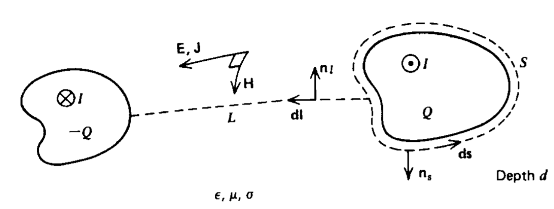
Figure 6-33 The electric and magnetic fields in the two-dimensional homogeneous charge and current-free region between hollow electrodes can be derived from a scalar potential that obeys Laplace's equation. The electric field lines are along the magnetic potential lines and vice versa so E and H are perpendicular. The inductance-capacitance product is then a constant.