6.6: The Energy Method for Forces

The Principle of Virtual Work

In Section 6-5-1 we calculated the energy stored in a current-carrying loop by two methods. First we calculated the electric energy input to a loop with no mechanical work done. We then obtained the same answer by computing the mechanical work necessary to move a current-carrying loop in an external field with no further electrical inputs. In the most general case, an input of electrical energy can result in stored energy dW and mechanical work by the action of a force \(f_{x}\) causing a small displacement dx:

\[i d \Phi = d W + f_{x} dx \]

If we knew the total energy stored in the magnetic field as a function of flux and position, the force is simply found as

\[f_{x} = - \frac{\partial W}{\partial x} \bigg|_{\Phi} \]

We can easily compute the stored energy by realizing that no matter by what process or order the system is assembled, if the final position x and flux \(\Phi\) are the same, the energy is the same. Since the energy stored is independent of the order that we apply mechanical and electrical inputs, we choose to mechanically assemble a system first to its final position x with no electrical excitations so that \(\Phi = 0\). This takes no work as with zero flux there is no force of electrical origin. Once the system is mechanically assembled so that its position remains constant, we apply the electrical excitation to bring the system to its final flux value. The electrical energy required is

\[W = \int_{x \textrm{ const}} i d \Phi \]

For linear materials, the flux and current are linearly related through the inductance that can now be a function of x because the inductance depends on the geometry:

\[i = \Phi/L (x) \]

Using (4) in (3) allows us to take the inductance outside the integral because x is held constant so that the inductance is also constant:

\[W = \frac{1}{L(x)} \int_{0}^{\Phi} \Phi d \Phi \\ = \frac{\Phi^{2}}{2 L (x)} = \frac{1}{2} L (x) i^{2} \]

The stored energy is the same as found in Section 6-5-2 even when mechanical work is included and the inductance varies with position.

To find the force on the moveable member, we use (2) with the energy expression in (5), which depends only on flux and position:

\[f_{x} = - \frac{\partial W}{\partial x} \bigg|_{\Phi} \\ = - \frac{\Phi^{2}}{2} \frac{d [1/L(x)]}{dx} \\ = \frac{1}{2} \frac{\Phi^{2}}{L^{2}(x)} \frac{dL(x)}{dx} \\ = \frac{1}{2} i^{2} \frac{dL(x)}{dx} \]

Circuit Viewpoint

This result can also be obtained using a circuit description with the linear flux-current relation of (4):

\[v = \frac{d \Phi}{dt} = L (x) \frac{di}{dt} + i \frac{dL(x)}{dt} \\ = L (x) \frac{di}{dt} + i \frac{dL(x)}{dx} \frac{dx}{dt} \]

The last term, proportional to the speed of the moveable member, just adds to the usual inductive voltage term. If the geometry is fixed and does not change with time, there is no electromechanical coupling term.

The power delivered to the system is

\[p = vi = i \frac{d}{dt} [L(x)i] \]

which can be expanded as

\[p = \frac{d}{dt}(\frac{1}{2}L(x)i^{2}) + \frac{1}{2}i^{2} \frac{dL(x)}{dx} \frac{dx}{dt} \]

This is in the form

\[p = \frac{dW}{dt} + f_{x} \frac{dx}{dt}, \: \left \{ \begin{matrix} W = \frac{1}{2} L (x) i^{2} \\ f_{x} = \frac{1}{2} i^{2} \frac{dL(x)}{dx} \end{matrix} \right. \]

which states that the power delivered to the inductor is equal to the sum of the time rate of energy. stored and mechanical power performed on the inductor. This agrees with the energy method approach. If the inductance does not change with time because the geometry is fixed, all the input power is stored. as potential energy \(W\).

Example \(\PageIndex{2}\) MAGNETIC FIELDS AND FORCES

(a) Relay

Find the force on the moveable slug in the magnetic circuit shown in Figure 6-34.

SOLUTION

---

It is necessary to find the inductance of the system as a function of the slug's position so that we can use (6). Because of the infinitely permeable core and slug, the \(\textbf{H}\) field is non­zero only in the air gap of length \(x\). We use Ampere's law to obtain

\[ H=NI/x \nonumber \]

The flux through the gap

\[ \Phi =\mu _{0}NIA/x  \nonumber \]

is equal to the flux through each turn of the coil yielding the inductance as

\[ L(x)=\frac{N \Phi}{I}=\frac{\mu_0 N^2 A}{x} \nonumber \]

Figure 6-34 The magnetic field exerts a force on the moveable member in the relay pulling it into the magnetic circuit.

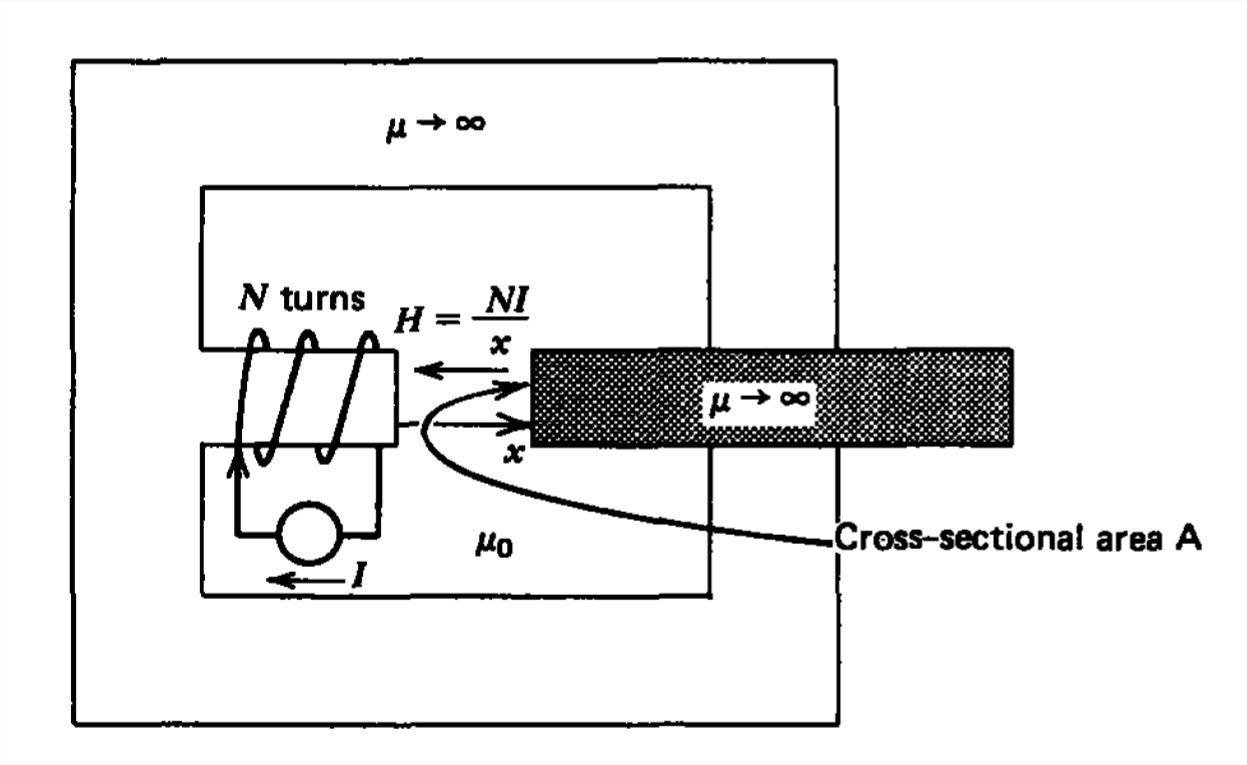
The force is then

\[ \begin{aligned}
f_x & =\frac{1}{2} I^2 \frac{d L(x)}{d x} \\
& =-\frac{\mu_o N^2 A I^2}{2 x^2}
\end{aligned}  \]

The minus sign means that the force is opposite to the direc­tion of increasing \(x\), so that the moveable piece is attracted to the coil.

(b) One Turn Loop

Find the force on the moveable upper plate in the one turn loop shown in Figure 6-35.

SOLUTION

---

The current distributes itself uniformly as a surface current \(K=I/D\) on the moveable plate. If we neglect nonuniform field effects near the corners, the \(\textbf{H}\) field being tangent to the conductors just equals \(K\):

\[ H_{z}=I/D   \nonumber \]

The total flux linked by the current source is then

\[ \begin{aligned}
\Phi & =\mu_0 H_z x l \\
& =\frac{\mu_0 x l}{D} I
\end{aligned}  \]

which gives the inductance as

\[ L\left ( x \right )=\frac{\Phi }{I}=\frac{\mu _{0}xl}{D}  \nonumber \]

Figure 6-35 The magnetic force on a current-carrying loop tends to expand the loop,

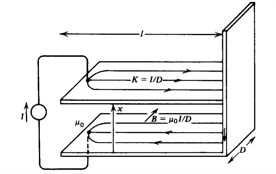
The force is then constant

\begin{aligned}
f_x & =\frac{1}{2} I^2 \frac{d L(x)}{d x} \\
& =\frac{1}{2} \frac{\mu_0 l I^2}{D}
\end{aligned}

Magnetization Force

A material with permeability \(\mu \) is partially inserted into the magnetic circuit shown in Figure 6-36. With no free current in the moveable material, the \(x\)-directed force density from Section 5-8-1 is

\[\begin{align}F_{x}&=\mu _{0}\left ( \textbf{M}\cdot \nabla \right )H_{x} \\ &
=\left ( \mu -\mu _{0} \right )\left ( \textbf{H}\cdot \nabla \right )H_{x} \nonumber\\ &
=\left ( \mu -\mu _{0} \right )\left ( H_{x}\frac{\partial H_{x}}{\partial x}+H_{y}\frac{\partial H_{x}}{\partial y} \nonumber \right )\end{align} \]

where we neglect variations with \(z\). This force arises in the fringing field because within the gap the magnetic field is essentially uniform:

\[H_{y}=NI/s \]

Because the magnetic field in the permeable block is curl free,

\[\nabla \times \textbf{H}=0\Rightarrow \frac{\partial H_{x}}{\partial y}=\frac{\partial H_{y}}{\partial x} \]

Figure 6-36 - A permeable material tends to be pulled into regions of higher magnetic field.

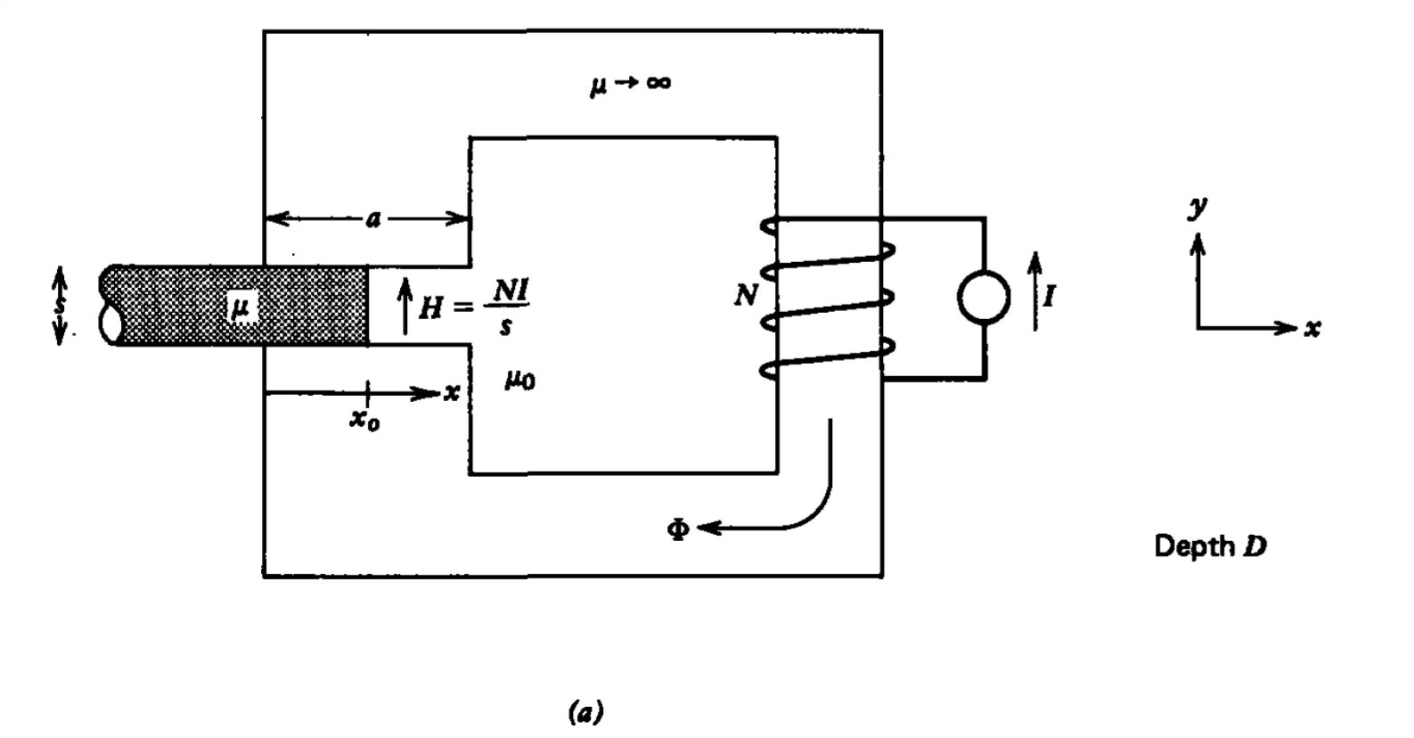
(11) can be rewritten as

\[F_{x}=\frac{\left ( \mu -\mu _{0} \right )}{2}\frac{\partial }{\partial x}\left ( H_{x}^{2}+H_{y}^{2} \right ) \]

The total force is then

\[\begin{align}f_{x}&=sD\int_{-\infty }^{x_{0}}F_{x}\,dx  \\ &
=\frac{\left ( \mu -\mu _{0} \right )}{2}sD\left ( H_{x}^{2}+H_{y}^{2} \right )\bigg|_{-\infty }^{x_{0}} \nonumber \\ &
=\frac{\left ( \mu -\mu _{0} \right )}{2}\frac{N^{2}I^{2}D}{s} \nonumber \end{align} \]

where the fields at \(x=-\infty \) are zero and the field at \(x=x_{0}\) is given by (12). High permeability material is attracted to regions of stronger magnetic field. It is this force that causes iron materials to be attracted towards a magnet. Diamagnetic materials \(\left ( \mu < \mu _{0} \right )\) will be repelled.

This same result can more easily be obtained using (6) where the flux through the gap is

\[\Phi =HD\left [ \mu x+\mu _{0}\left ( a-x \right ) \right ]=\frac{NID}{s}\left [ \left ( \mu -\mu _{0} \right )x+a\mu _{0} \right ] \]

so that the inductance is

\[L=\frac{N\Phi }{I}=\frac{N^{2}D}{s}\left [ \left ( \mu -\mu _{0} \right )+a\mu _{0} \right ] \]

Then the force obtained using (6) agrees with (15)

\[\begin{align} f_{x}&=\frac{1}{2}I^{2}\frac{dL\left (x \right )}{dx} \\ &=\frac{\left ( \mu -\mu _{0} \right )}{2s}N^{2}I^{2}D \nonumber \end{align} \]