4.6: Unbalanced Faults

A very common application of symmetrical components is in calculating currents arising from unblanced short circuits. For three-phase systems, the possible unbalanced faults are:

1. Single line-ground,
2. Double line-ground,
3. Line-line.

These are considered separately.

Single Line-To-Ground Fault

The situation is as shown in Figure 10

The system in this case consists of networks connected to the line on which the fault occurs. The point of fault itself consists of a set of terminals (which we might call “a,b,c”). The fault sets,

Figure 9: Zero Sequence Network: Wye-Delta Connection, Ungrounded or Delta-Delta

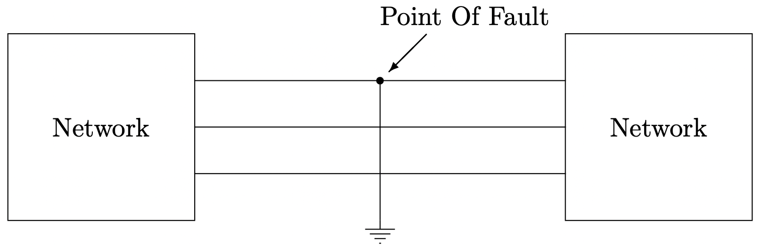Figure 10: Schematic Picture Of A Single Line-To-Ground Fault

at this point on the system:

\(\ \begin{aligned}
\underline{V}_{a} &=0 \\
\underline{I}_{b} &=0 \\
\underline{I}_{c} &=0
\end{aligned}\)

Now: using the inverse of the symmetrical component transformation, we see that:

\[\ \underline{V}_{1}+\underline{V}_{2}+\underline{V}_{0}=0\label{58} \]

And using the transformation itself:

\[\ \underline{I}_{1}=\underline{I}_{2}=\underline{I}_{0}=\frac{1}{3} \underline{I}_{a}\label{59} \]

Together, these two expressions describe the sequence network connection shown in Figure 11. This connection has all three sequence networks connected in series.

Double Line-To-Ground Fault

If the fault involves phases b, c, and ground, the “terminal” relationship at the point of the fault is:

\(\ \begin{array}{l}
\underline{V}_{b}=0 \\
\underline{V}_{c}=0 \\
\underline{I}_{a}=0
\end{array}\)

Then, using the sequence transformation:

\(\ \underline{V}_{1}=\underline{V}_{2}=\underline{V}_{0}=\frac{1}{3} \underline{V}_{a}\)

Combining the inverse transformation:

\(\ \underline{I}_{a}=\underline{I}_{1}+\underline{I}_{2}+\underline{I}_{0}=0\)

These describe a situation in which all three sequence networks are connected in parallel, as shown in Figure 12.

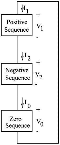Figure 11: Sequence Connection For A Single-Line-To-Ground Fault

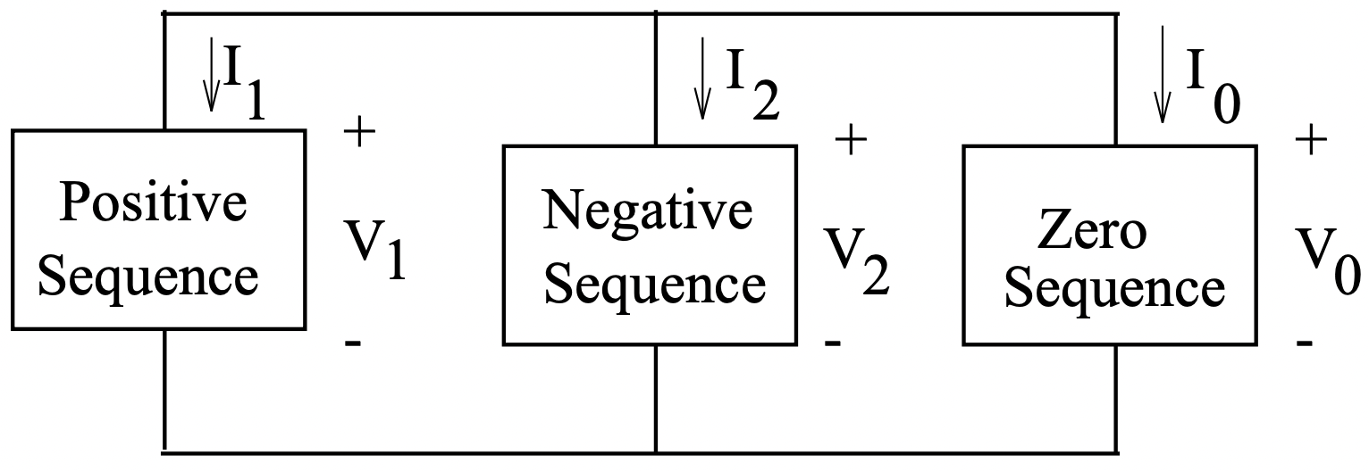Figure 12: Sequence Connection For A Double-Line-To-Ground Fault

Line-Line Fault

If phases b and c are shorted together but not grounded,

\(\ \begin{aligned}
\underline{V}_{b} &=\underline{V}_{c} \\
\underline{I}_{b} &=-\underline{I}_{c} \\
\underline{I}_{a} &=0
\end{aligned}\)

Expressing these in terms of the symmetrical components:

\(\ \begin{aligned}
\underline{V}_{1} &=\underline{V}_{2} \\
&=\frac{1}{3}\left(\underline{a}+\underline{a}^{2}\right) \underline{V}_{b} \\
\underline{I}_{0} &=\underline{I}_{a}+\underline{I}_{b}+\underline{I}_{c} \\
&=0 \\
\underline{I}_{a} &=\underline{I}_{1}+\underline{I}_{2}\\
&=0
\end{aligned}\)

These expressions describe a parallel connection of the positive and negative sequence networks, as shown in Figure 13.

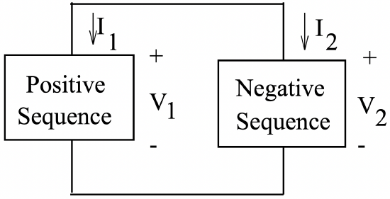Figure 13: Sequence Connection For A Line-To-Line Fault

Example Of Fault Calculations

In this example, the objective is to determine maximum current through the breaker B due to a fault at the location shown in Figure 14. All three types of unbalanced fault, as well as the balanced fault are to be considered. This is the sort of calculation that has to be done whenever a line is installed or modified, so that protective relaying can be set properly.

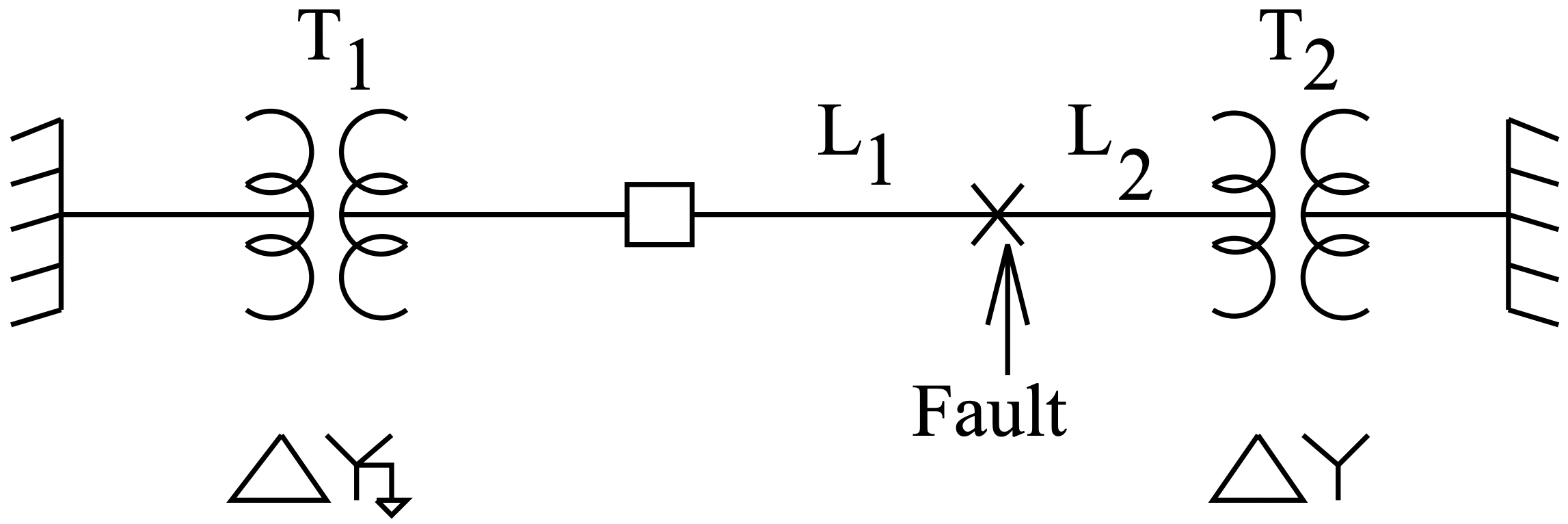Figure 14: One-Line Diagram For Example Fault

Parameters of the system are:

System Base Voltage	138 kV
System Base Power	100 MVA
Transformer \(\ T_{1}\) Leakage Reactance	.1 per-unit
Transformer \(\ T_{2}\) Leakage Reactance	.1 per-unit
Line \(\ L_{1}\) Positive And Negative Sequence Reactance	j.05 per-unit
Line \(\ L_{1}\) Zero Sequence Impedance	j.1 per-unit
Line \(\ L_{2}\) Positive And Negative Sequence Reactance	j.02 per-unit
Line \(\ L_{2}\) Zero Sequence Impedance	j.1 per-unit

The fence-like symbols at either end of the figure represent “infinite buses”, or positive sequence voltage sources.

The first step in this is to find the sequence networks. These are shown in Figure 15. Note that they are exactly like what we would expect to have drawn for equivalent single phase networks. Only the positive sequence network has sources, because the infinite bus supplies only positive sequence voltage. The zero sequence network is open at the right hand side because of the deltawye transformer connection there.

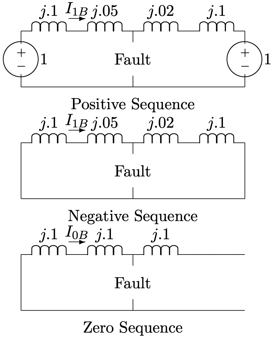Figure 15: Sequence Networks

Symmetrical Fault

For a symmetrical (three-phase) fault, only the positive sequence network is involved. The fault shorts the network at its position, so that the current is:

\(\ \underline{i}_{1}=\frac{1}{j .15}=-j 6.67 \text { per }-\text { unit }\)

Single Line-Ground Fault

For this situation, the three networks are in series and the situation is as shown in Figure 16

The current \(\ \underline{i}\) shown in Figure 16 is a total current, and is given by:

\(\ \underline{i}=\frac{1}{2 \times(j .15 \| j .12)+j .2}=-j 3.0\)

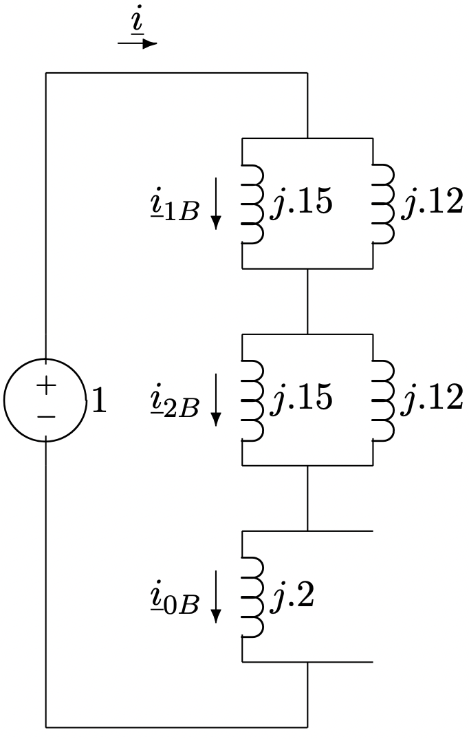Figure 16: Completed Network For Single Line-Ground Fault

Then the sequence currents at the breaker are:

\(\ \begin{aligned}
\underline{i}_{1 B} &=\underline{i}_{2 B} \\
&=\underline{i} \times \frac{j .12}{j .12+j .15} \\
&=-j 1.33 \\
\underline{i}_{0 B} &=\underline{i} \\
&=-j 3.0
\end{aligned}\)

The phase currents are re-constructed using:

\(\ \begin{aligned}
\underline{i}_{a} &=\underline{i}_{1 B}+\underline{i}_{2 B}+\underline{i}_{0 B} \\
\underline{i}_{b} &=\underline{a}^{2} \underline{i}_{1 B}+\underline{ai}_{2 B}+\underline{i}_{0 B} \\
\underline{i}_{c} &=\underline{ai}_{1 B}+\underline{a}^{2} \underline{i}_{2 B}+\underline{i}_{0 B}
\end{aligned}\)

These are:

\(\ \begin{aligned}
i_{a} &=-j 5.66 & & \text { per-unit } \\
\underline{i}_{b} &=-j 1.67 & & \text { per-unit } \\
\underline{i}_{c} &=-j 1.67 & & \text { per-unit }
\end{aligned}\)

Double Line-Ground Fault

For the double line-ground fault, the networks are in parallel, as shown in Figure 17.

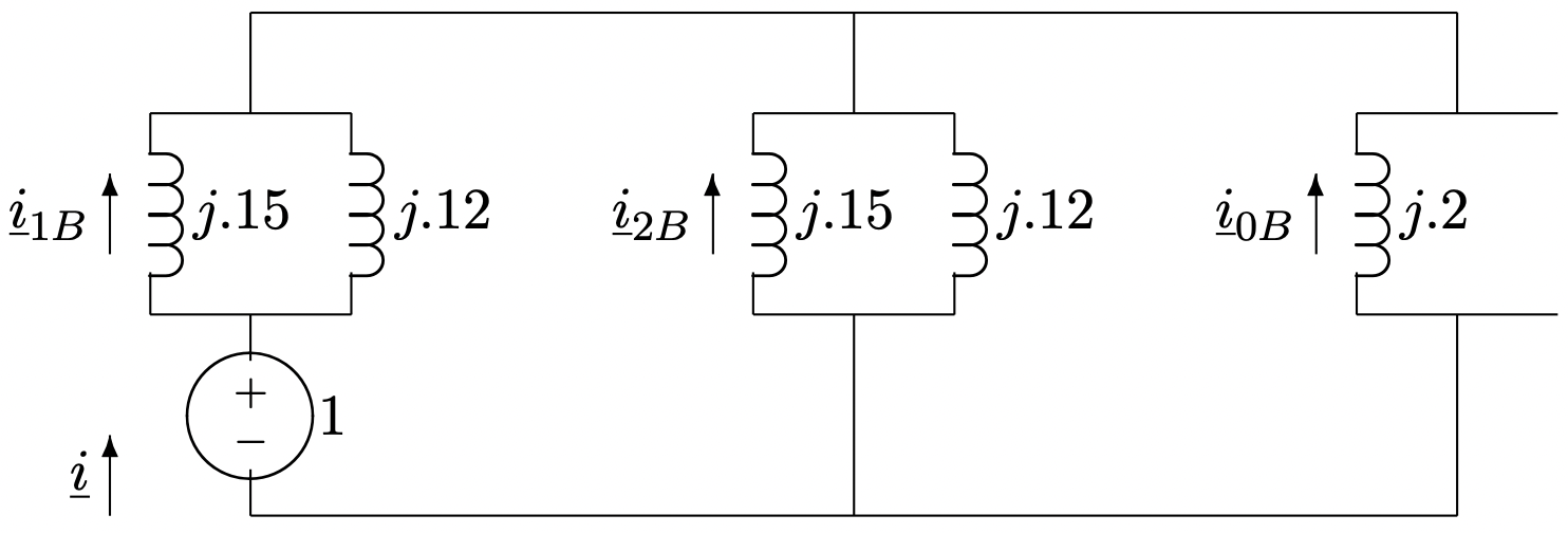Figure 17: Completed Network For Double Line-Ground Fault

To start, find the source current \(\ \underline{i}\):

\(\ \begin{aligned}
\underline{i} &=\frac{1}{j(.15|| \cdot 12)+j(.15|| .12|| .2)} \\
&=-j 8.57
\end{aligned}\)

Then the sequence currents at the breaker are:

\(\ \begin{aligned}
\underline{i}_{1 B} &=\underline{i} \times \frac{j .12}{j .12+j .15} \\
&=-j 3.81 \\
\underline{i}_{2 B} &=-\underline{i} \times \frac{j .12 \| j .2}{j .12 \| j .2+j .15} \\
&=j 2.86 \\
\underline{i}_{0 B} &=\underline{i} \times \frac{j .12 \| j .15}{j .2+j .12 \| j .15} \\
&=j 2.14
\end{aligned}\)

Reconstructed phase currents are:

\(\ \begin{aligned}
\underline{i}_{a} &=j 1.19 \\
\underline{i}_{b} &=\underline{i}_{0 B}-\frac{1}{2}\left(\underline{i}_{1 B}+\underline{i}_{2 B}\right)-\frac{\sqrt{3}}{2} j\left(\underline{i}_{1 B}-\underline{i}_{2 B}\right) \\
&=j 2.67-5.87 \\
\underline{i}_{c} &=\underline{i}_{0 B}-\frac{1}{2}\left(\underline{i}_{1 B}+\underline{i}_{2 B}\right)+\frac{\sqrt{3}}{2} j\left(\underline{i}_{1 B}-\underline{i}_{2 B}\right) \\
&=j 2.67+5.87 \\
|\underline{i}_{a} \mid &=1.19 \quad \text { per-unit } \\
\left|\underline{i}_{b}\right| &=6.43 \quad \text { per-unit } \\
\left|i_{c}\right| &=6.43 \quad \text { per-unit }
\end{aligned}\)

Line-Line Fault

The situation is even easier here, as shown in Figure 18

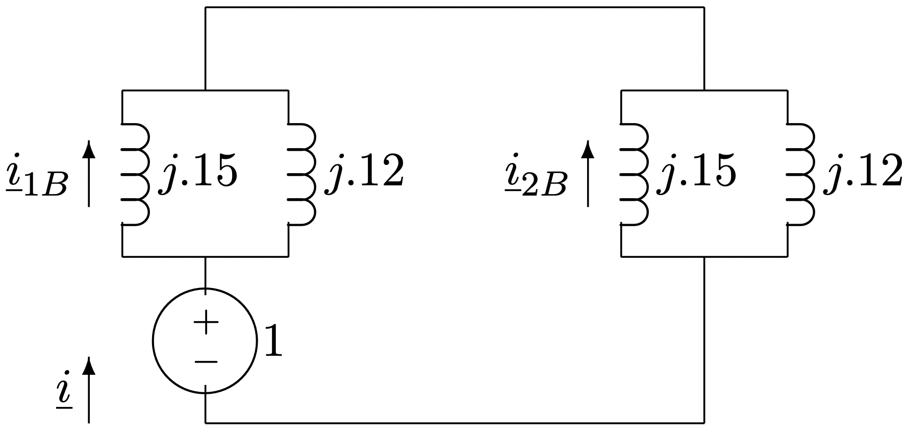Figure 18: Completed Network For Line-Line Fault

The source current \(\ \underline{i}\) is:

\(\ \begin{aligned}
\underline{i} &=\frac{1}{2 \times j(.15 \| .12)} \\
&=-j 7.50
\end{aligned}\)

and then:

\(\ \begin{aligned}
\underline{i}_{1 B} &=-\underline{i}_{2 B} \\
&=i \frac{j .12}{j .12+j .15} \\
&=-j 3.33
\end{aligned}\)

Phase currents are:

\(\ \begin{aligned}
\underline{i}_{a} &=0 \\
\underline{i}_{b} &=-\frac{1}{2}\left(\underline{i}_{1 B}+\underline{i}_{2 B}\right)-j \frac{\sqrt{3}}{2}\left(\underline{i}_{1 B}-\underline{i}_{2 B}\right) \\
\left|\underline{i}_{b}\right| &=5.77 \quad \text { per-unit } \\
\left|i_{c}\right| &=5.77 \quad \text { per-unit }
\end{aligned}\)

Conversion To Amperes

Base current is:

\(\ I_{B}=\frac{P_{B}}{\sqrt{3} V_{B l-l}}=418.4 A\)

Then current amplitudes are, in Amperes, RMS:

	Phase A	Phase B	Phase C
Three-Phase Fault	2791	2791	2791
Single Line-Ground, \(\ \phi_{a}\)	2368	699	699
Double Line-Ground, \(\ \phi_{b}, \phi_{c}\)	498	2690	2690
Line-Line, \(\ \phi_{b}, \phi_{c}\)	0	2414	2414