5.5: Example

Consider the system shown in Figure 1. This simple system has five buses (numbered 1 through 5) and four lines. Two of the buses are connected to generators, two to loads and bus 5 is the “swing bus”, represented as an “infinite bus”, or voltage supply.

For the purpose of this excercise, assume that the line impedances are:

\[\ \begin{array}{l}
\mathbf{Z}_{0}=.05+j .1 \\
\mathbf{Z}_{1}=.05+j .05 \\
\mathbf{Z}_{2}=.15+j .2 \\
\mathbf{Z}_{3}=.04+j .12
\end{array}\label{12} \]

We also specify real power and voltage magnitude for the generators and real and reactive power for the loads:

• Bus 1: Real power is 1, voltage is 1.05 per–unit
• Bus 2: Real power is 1, voltage is 1.00 per–unit
• Bus 3: Real power is -.9 per–unit, reactive power is 0
• Bus 4: Real power is -1, reactive power is -.2 per–unit.

Note that load power is taken to be negative, for this simple–minded program assumes all power is measured into the network.

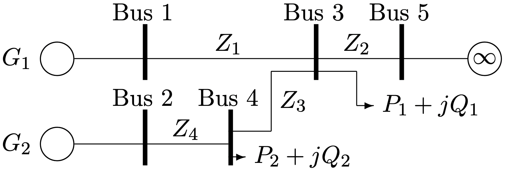Figure 1: Sample System

% Simple-Minded Load Flow Example

% First, impedances

Z1=.05+j*.1;

Z2=.05+j*.05;

Z3=.15+j*.2;

Z4=.04+j*.12;

% This is the node-incidence Matrix

NI=[1 0 0 0 ; 0 0 0 1 ; -1 1 1 0 ; 0 0 -1 -1 ; 0 -1 0 0];

% This is the vector of "known" voltage magnitudes

VNM = [1.05 1 0 0 1]’;

% And the vector of known voltage angles

VNA = [0 0 0 0 0]’;

% and this is the "key" to which are actually known

KNM = [1 1 0 0 1]’;

KNA = [0 0 0 0 1]’;

% and which are to be manipulated by the system

KUM = 1 - KNM;

KUA = 1 - KNA;

% Here are the known loads (positive is INTO network

% Use zeros for unknowns

P=[1 1 -.9 -1 0]’;

Q=[0 0 0 -.2 0]’;

% and here are the corresponding vectors to indicate

% which elements should be checked in error checking

PC = [1 1 1 1 0]’;

QC = [0 0 1 1 0]’;

Check = KNM + KNA + PC + QC;

% Unknown P and Q vectors

PU = 1 - PC;

QU = 1 - QC;

fprintf(’Here is the line admittance matrix:\n’);

Y=[1/Z1 0 0 0;0 1/Z2 0 0;0 0 1/Z3 0;0 0 0 1/Z4]

% Construct Node-Admittance Matrix

fprintf(’And here is the bus admittance matrix\n’)

YN=NI*Y*NI’

% Now: here are some starting voltage magnitudes and angles

VM = [1.05 1 .993 .949 1]’;

VA = [.0965 .146 .00713 .0261 0]’;

% Here starts a loop

Error = 1;

Tol=1e-10;

N = length(VNM);

% Construct a candidate voltage from what we have so far

VMAG = VNM .* KNM + VM .* KUM;

VANG = VNA .* KNA + VA .* KUA;

V = VMAG .* exp(j .* VANG);

% and calculate power to start

I = (YN*V);

PI = real(V .* conj(I));

QI = imag(V .* conj(I));

%pause

while(Error>Tol);

for i=1:N, % Run through all of the buses

% What we do depends on what bus!

if (KUM(i) == 1) & (KUA(i) == 1), % don’t know voltage magnitude or angle

pvc= (P(i)-j*Q(i))/conj(V(i));

for n=1:N,

if n ~=i, pvc = pvc - (YN(i,n) * V(n)); end

end

V(i) = pvc/YN(i,i);

elseif (KUM(i) == 0) & (KUA(i) == 1), % know magnitude but not angle

% first must generate an estimate for Q

Qn = imag(V(i) * conj(YN(i,:)*V));

pvc= (P(i)-j*Qn)/conj(V(i));

for n=1:N,

if n ~=i, pvc = pvc - (YN(i,n) * V(n)); end

end

pv=pvc/YN(i,i);

V(i) = VM(i) * exp(j*angle(pv));

end % probably should have more cases

end % one shot through voltage list: check error

% Now calculate currents indicated by this voltage expression

I = (YN*V);

% For error checking purposes, compute indicated power

PI = real(V .* conj(I));

QI = imag(V .* conj(I));

% Now we find out how close we are to desired conditions

PERR = (P-PI) .* PC;

QERR = (Q-QI) .* QC;

Error = sum(abs(PERR) .^2 + abs(QERR) .^2);

end

fprintf(’Here are the voltages\n’)

V

fprintf(’Real Power\n’)

P

fprintf(’Reactive Power\n’)

Q