9.3: Physical Picture- Current Sheet Description

Consider this simple picture. The ‘machine’ consists of a cylindrical rotor and a cylindrical stator which are coaxial and which have sinusoidal current distributions on their surfaces: the outer surface of the rotor and the inner surface of the stator.

The ‘rotor’ and ‘stator’ bodies are made of highly permeable material (we approximate this as being infinite for the time being, but this is something that needs to be looked at carefully later). We also assume that the rotor and stator have current distributions that are axially (z) directed and sinusoidal:

\(\ \begin{array}{l}
K_{z}^{S}=K_{S} \cos p \theta \\
K_{z}^{R}=K_{R} \cos p(\theta-\phi)
\end{array}\)

Here, the angle \(\ \phi\) is the physical angle of the rotor. The current distribution on the rotor goes along. Now: assume that the air-gap dimension g is much less than the radius: \(\ g<<R\). It is not

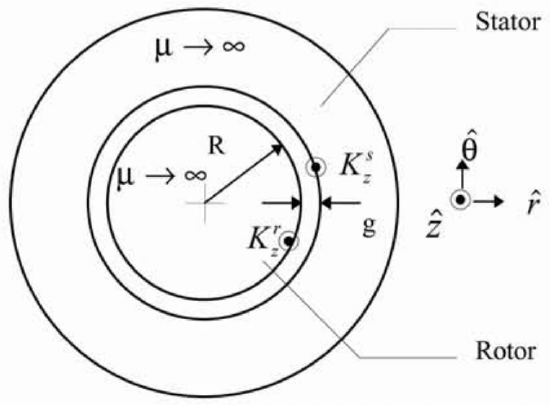Figure 1: Elementary Machine Model: Axial View

difficult to show that with this assumption the radial flux density Br is nearly uniform across the gap (i.e. not a function of radius) and obeys:

\(\ \frac{\partial B_{r}}{\partial \theta}=-\mu_{0} \frac{K_{z}^{S}+K_{z}^{R}}{g}\)

Then the radial magnetic flux density for this case is simply:

\(\ B_{r}=-\frac{\mu_{0} R}{p g}\left(K_{S} \sin p \theta+K_{R} \sin p(\theta-\phi)\right)\)

Now it is possible to compute the traction on rotor and stator surfaces by recognizing that the surface current distributions are the azimuthal magnetic fields: at the surface of the stator, \(\ H_{\theta}=-K_{z}^{S}\) and at the surface of the rotor, \(\ H_{\theta}=K_{z}^{R}\). So at the surface of the rotor, traction is:

\(\ \tau_{\theta}=T_{r \theta}=-\frac{\mu_{0} R}{p g}\left(K_{S} \sin p \theta+K_{R} \sin p(\theta-\phi)\right) K_{R} \cos p(\theta-\phi)\)

The average of that is simply:

\(\ <\tau_{\theta}>=-\frac{\mu_{0} R}{2 p g} K_{S} K_{R} \sin p \phi\)

The same exercise done at the surface of the stator yields the same results (with opposite sign). To find torque, use:

\(\ T=2 \pi R^{2} \ell<\tau_{\theta}>=\frac{\mu_{0} \pi R^{3} \ell}{p g} K_{S} K_{R} \sin p \phi\)

We can pause here to make a few observations:

1. For a given value of surface currents Ks and Kr, torque goes as the fourth power of linear dimension. The volume of the machine goes as the third power, so this implies that torque capability goes as the 413 power of machine volume. Actually, this understates the situation since the assumed surface current densities are the products of volume current densities and winding depth, which one would expect to increase with machine size. Thus machine torque (and power) densities tend to increase somewhat faster with size.

2. \(\ K_{z}^{S}=K_{S} \cos (p \theta-\omega t)\)

   and this pulls the rotor along.

3. For a given pair of current distributions there is a maximum torque that can be sustained, but as long as the torque that is applied to the rotor is less than that value the rotor will adjust to the correct angle.